Jan 22, 2018 · post
Exploring Recommendation Systems
While we commonly associate recommendation systems with e-commerce, their application extends to any decision-making problem which requires pairing two types of things together. To understand why recommenders don’t always work as well as we’d like them to, we set out to build some basic recommendation systems using publicly available data.
Data
The first ingredient for building a recommendation system is user interaction data. We experimented with two different datasets, one from Flickr and one from Amazon. The Flickr dataset contains interactions between users and photos that they liked; the Amazon dataset contains user ratings on books. Both datasets are time-stamped. The Flickr dataset has positive class data only (i.e. liked photos), while the Amazon dataset has granular ratings data ranging from 1 to 5.
In general, user interaction data is sparse, since a single user would only have interacted with a small subset of items (think about how many movies you have rated on Netflix). In addition, users tend to rate good items only, leading to class imbalance. For datasets with granular ratings data, not only is it hard for a user to differentiate 2 from 3, a 3 could also mean different things to different users.
In recommendation systems, it is important to remove both users who have interacted with many items and items that have many ratings. Intuitively, users who like many items do not add any useful information to our system, as they are not selective enough. Similarly, items that many users like will tend to be overly recommended. To clean our dataset, we filtered out these cases. We then split the dataset into two (training and testing), using a cutoff timestamp.
Building the Recommender
The goal of a recommendation system is to use historical interaction data to recommend a new pairing (user and item) for the future. There are two approaches. The first approach predicts an actual rating for a user-item pair and recommends the highest rated item for that user. The second approach predicts a ranking of items and recommends the highest ranked item for a user. Our experiment focuses on the first approach. The recommenders are evaluated using standard metrics such as area under curve (AUC) and root mean squared error (RMSE).
AUC computes the area under the ROC curve for classification problems, and a larger number is better. The ROC curve plots the true positive rate against the false positive rate. We want a classifier that correctly identifies as many positive instances as are available, with a very low percentage of negative instances incorrectly classified as positive. As a result, the ROC curve of a perfect classifier will go straight up the y axis (true positive rate) and then along the x axis (false positive rate). A classifier with no power will sit on the x=y diagonal. RMSE computes how far the predicted value is from the actual value.
Basic photo recommendation system
To quickly get a recommender up and running, we used a Python scikit called SURPRISE. The package has various built-in recommendation algorithms including ones based on neighborhood approach and matrix factorization. Neighborhood approach finds a group of users who are similar to you and assumes that you share the same item preferences. The algorithm then recommends to you items that these users have liked. Matrix factorization represents users and items using a set of factors and predicts user preference for items using a linear combination of these factors. Because a recommender needs to know both what a user liked and disliked, we used heuristics to infer negative ratings for the Flickr dataset. (An example heuristic is to assume that x number of photos before the liked photo are disliked.)
With both positive and negative ratings, we were ready to plug our data into SURPRISE. To do so, we transformed it into a text file that provides four pieces of information {userid, photoid, rating, timestamp}, where a rating is either a 1 or 5.
The following code snippet shows how custom datasets can be defined and used in SURPRISE.
from surprise import Dataset
from surprise import Reader

train_file = os.path.expanduser(data_path + 'train.data')
test_file = os.path.expanduser(data_path + 'test.data')
reader = Reader(line_format='user item rating timestamp', sep=';')
data = Dataset.load_from_folds([(train_file, test_file)], reader=reader)
Training a model and getting a prediction is straightforward.
from surprise import dump
from surprise import KNNBasic
from surprise.accuracy import rmse

algo = KNNBasic(sim_options=sim_options, min_k=3)
for trainset, testset in data.folds():
    algo.train(trainset)
    predictions = algo.test(testset)
    rmse(predictions)
    dump('./dump_KNN', predictions, trainset, algo)
The ROC curve for our system was underwhelming - it is very close to the diagonal line because there is not enough information in the interaction matrix.
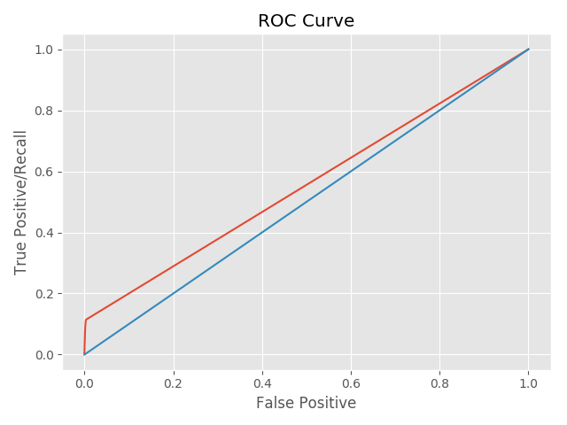
Photo recommender with Tags
Could we build a better recommendation system if we made use of the tag information that comes for free with the Flickr dataset? Instead of describing a photo using its id (a series of numbers), we used tags like sunset, bridge, Brooklyn. Why? First, by doing so, we hoped to add more information to the interaction matrix. Second, our basic photo recommender was unable to recommend a new photo because it did not have any historical interaction information. Since it did not know who had interacted with this photo and what the outcome of the interaction was, it did not know how to recommend this new item. (This is known as the cold start problem.) By adding tags, we built a system that understands the content of what it is recommending. With this understanding comes the ability to recommend items that it has never seen before. A new photo is no longer new to the system; it can be represented by a set of tags that the system has seen before.
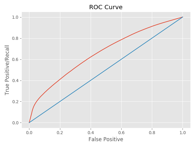
When we describe a photo with a set of tags, each column of the input matrix is now a tag (vs a photo id). As such, the size of the input matrix becomes much larger. For each user, the recommender returns a set of tags and their corresponding scores. To get back a photo recommendation, these tag scores need to be converted to photo scores. For each photo, we compute its score by i) comparing the recommended tags to the set of tags representing the photo, ii) finding the common tags between them, iii) adding up the scores for the common tags and iv) normalizing by the number of common tags. All photos are ranked using this score and the top one is recommended. Once tag information is incorporated, our ROC curve looked much better!
Basic book recommendation system
Our recommender based on Flickr’s dataset required inferred negative ratings. Amazon’s user rating dataset, on the other hand, provides rating information ranging from 1 to 5. We tested two recommenders on this dataset: the first was a recommender we built using Python’s scikit-learn package; the second was a recommender put together using Spotlight, a PyTorch based recommendation package. In our scikit-learn implementation we incorporated both matrix factorization and neighborhood-based algorithms. In the Spotlight recommender, we built an engine using matrix factorization since Spotlight does not support neighborhood based-approaches. All recommenders are evaluated using RMSE.
We cleaned and separated the Amazon dataset into training and testing sets using the same approach as we did with the Flickr dataset. From here, we transformed the input data into an interaction matrix for our sklearn-based recommender. Each row in the interaction matrix represents a user and each column represents a book. For Spotlight, this interaction matrix is converted into a custom interactions object. This object takes in three arrays: user ID, book ID, and ratings information. The user ID is the row index for our interaction matrix, the book ID is the column index, and the rating information is the value of the interaction matrix. Here is the code snippet.
from spotlight.interactions import Interactions
interactions = Interactions(np.asarray(userid, dtype=np.int32),
	       		    np.asarray(bookid, dtype=np.int32),
                            np.asarray(ratings_all, dtype=np.float32))
Training and scoring the model is a two liner.
from spotlight.factorization.explicit import ExplicitFactorizationModel
from spotlight.evaluation import rmse_score

model = ExplicitFactorizationModel(n_iter=1)
model.fit(sp_train[0])
rmse = rmse_score(model, sp_test[0])  # 0.62
Similar to our results with the Flickr dataset, the initial results were underwhelming, but expected for a system built using only user and book ratings information.
Book Recommender with Subject
What if we added some content information to the books? In the Flickr dataset, each photo already has a set of tags associated with it; content information is free! For the Amazon dataset, we obtained subject information using the open library API. This allowed us to identify a book using its subject. Each column in our interaction matrix is now a subject rather than a book ID. Since multiple books can be mapped to the same subject, our input matrix is smaller and denser. (This is in contrast to the Flickr dataset, where adding content information expanded the input matrix.) Ratings that a user assigned for books with the same subject are aggregated into a single rating for that particular subject. To obtain a recommended rating on a book, we mapped the book to its subject and read off that recommendation. With subject information, the RMSE improved by approximately 2-fold across the board! Unfortunately, we also saw that most of the algorithms do not work since they perform worse than a random recommender when we use RMSE as a metric.
| Algorithm | RMSE |
|---|---|
| NMF (ID) | 0.84 |
| NMF (Subject) | 0.46 |
| Neighborhood (ID) | 0.84 |
| Neighborhood (Subject) | 0.44 |
| Spotlight MF (ID) | 0.62 |
| Spotlight MF (Subject) | 0.27 |
| Random | 0.38 |
What we learned
Raw material
Data makes all the difference. Traditional recommendation systems do not work well because of the sparsity problem. Each user only rates a small percentage of items in the universe, but recommendation systems rely on this weak signal to make decisions.
To make a better system we need a denser matrix in order to extract a stronger signal. In our example we used content information: tags for the Flickr dataset and subjects for the Amazon dataset. Both cases saw dramatic improvements.
Time-stamp information is also helpful because it makes the problem amenable to some deep learning techniques. As an example, the prototype we built to accompany our new Semantic Recommendations report uses deep features as a way of extending the factorization models.
Does a basic recommendation system work?
A recommendation system built using matrix factorization or neighborhood approaches trained on simple user-item interaction data is unlikely to give great recommendations. In our experiment with the Amazon dataset, these recommendation systems underperform a random system! Moreover, these systems suffer from the cold start problem - they rely on historical interaction data and cannot make recommendations on new items.
For more on recommendation systems, please see our new report! The Semantic Recommendations report explores the current state of recommendation systems, with a focus on how machines can better understand content. Armed with this newfound understanding, we look at how systems can bypass the cold start problem and expand their utility well beyond traditional e-commerce use cases.

