Jan 30, 2017 · post

The Algorithms Behind Probabilistic Programming

We recently introduced our report on probabilistic programming. The accompanying prototype allows you to explore the past and future of the New York residential real estate market.

This post gives a feel for the content in our report by introducing the algorithms and technology that make probabilistic programming possible. We’ll dive even deeper into these algorithms in conversation with the Stan Group Tuesday, February 7 at 1 pm ET/10am PT. Please join us!

Bayesian Inference

Probabilistic programming enables us to construct and fit probabilistic models in code. At its essence, Bayesian inference is a principled way to draw conclusions from incomplete or imperfect data, by interpreting data in light of prior knowledge of probabilities. As pretty much all real-world data is incomplete or imperfect in some way, it’s an important (and old!) idea.

Bayesian inference might be the way to go if you:

• want to make use of institutional knowledge (suspicions, beliefs, logical certainties) about the quantities you want to measure and predict, rather than learn solely from the data
• have several different datasets that you want to learn from
• need to quantify the probability of all possibilities, not just determine which is most likely
• want to do online learning (i.e., continually update your model as data arrives)
• want to do active learning (i.e., gather more information until your predictions reach some threshold of confidence)
• want to use data to decide if a more complicated model is justified
• need to explain your decisions to customers or regulators
• want to use a single model to answer several questions
• have sparse data with a shared or hierarchical structure

Many — perhaps most — analytics and product problems are like this. And the central idea of Bayesian inference is centuries old. Why, then, do relatively few data analysts, data scientists, and machine learning engineers use the approach?

The Algorithmic Building Blocks

The problem is that, until recently, the algorithms that make product and business problems tractable using Bayesian methods have been difficult to implement and computationally expensive to run. Probabilistic programming systems abstract away many of these difficulties by baking inference algorithms in as building blocks of the language. Morever, these algorithms are robust, so don’t require problem-specific hand-tuning.

One powerful example is sampling from an arbitrary probability distribution, which we need to do often (and efficiently!) when doing inference. The brute force approach, rejection sampling, is problematic because acceptance rates are low: as only a tiny fraction of attempts generate successful samples, the algorithms are slow and inefficient. See this post by Jeremey Kun for further details.

Until recently, the main alternative to this naive approach was Markov Chain Monte Carlo sampling (of which Metropolis Hastings and Gibbs sampling are well-known examples). If you used Bayesian inference in the 90s or early 2000s, you may remember BUGS (and WinBUGS) or JAGS, which used these methods. These remain popular teaching tools (see e.g. STATS331 by Brendon Brewer, our favorite elementary introduction to Bayesian data analysis). But MCMC samplers are often too slow for problems with rich structure or internet-scale data.

Bayesian inference research in the last 5-10 years has therefore focused on two new approaches that use clever ideas to make sure the sampler spends more time in regions of high probability, raising efficiency. Those are Hamiltonian Monte Carlo and Variational inference.

Hamiltonian Monte Carlo and the No U-Turn Sampler

Hamiltonian Monte Carlo (HMC) treats the probability distribution as a physical surface. It uses an elegant and computationally efficient idea from 19th-century physics to explore that surface using calculus, as if under the influence of gravity. This method doesn’t work for discrete parameters, but the user doesn’t need to differentiate functions by hand.

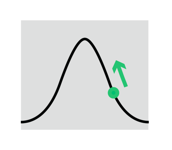
To use HMC, you need to tune a sensitive hyperparameter, which makes its application expensive and error-prone. The invention of the No U-Turn Sampler (NUTS), a robust algorithm that tunes this parameter automatically, was crucial for making probabilistic programming useful and practical.

Variational Inference and Automatic Differentation

Variational inference (VI) samples from a distribution by building a simple approximation of the distribution. That approximation is so simple that it can be sampled from directly, entirely circumventing the need for approximate sampling algorithms like MCMC or HMC.

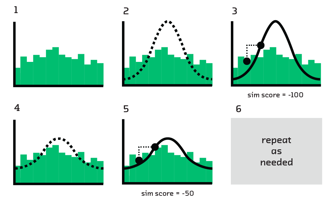
To do this, we start with simple distributions that we understand well (e.g., Gaussians) and perturb them until they match the real distribution from which we want to sample. The bulk of this work is done by stochastic gradient descent (SGD). Given its widespread use in machine learning (e.g., it’s used to train deep neural networks), SGD is well understood and optimized.

Converting a probabilistic model from a sampling approach to VI used to require complex math, making it hard for non-experts. Automatic Differentiation Variational Inference solves this problem by using automatic differentation (having computers take exact derivatives of arbitrary functions) to differentiate functions at the CPU instruction level, allowing a probability distribution to be explored efficiently.

Probabilistic Programming Languages

ADVI and HMC with NUTS are the two fundamental algorithmic innovations that have made probabilistic programming possible. Their inclusion in leading probabilistic programming environments (which can be traced back to these two blog posts from 2010) makes inference a one-liner. The end user doesn’t need to tune parameters or differentiate functions by hand. And because they’re built on Hamiltonian Monte Carlo or variational inference, they’re fast.

But fast and robust algorithms are not all that’s required to make Bayesian inference a practical proposition. Probabilistic programming languages also make life simpler by providing a concise syntax to define generative models using a library of built-in probability distributions. Probabilistic concepts are primitive objects defined in the core language. Specifying the model is therefore a declarative problem for the user, who declares what is known to be true and lets the language figure out how to derive conclusions.

The most popular probabilistic programming tools are Stan and PyMC3. Edward is a newcomer gaining a lot of attention. Stan experts Eric Novik and Daniel Lee will walk us through how Stan works and what problems they’ve used it to solve in our online event February 7.

For more on PyMC3 see our interview with Thomas Wiecki a PyMC3 core developer (and Director of Data Science at Quantopian). We also enjoyed Chris Fonnesbeck’s blog post that accompanied the recent official release of PyMC3.

In the report we go into more detail on the strengths and weaknesses of these two languages, and discuss some of the many other options. Whichever language you use, the claim of probabilistic programming - that it hides the complexity of Bayesian inference - is more true than ever.

– Mike