Nov 14, 2022 · post
Implementing CycleGAN
Introduction
This post documents the first part of a research effort to quantify the impact of synthetic data augmentation in training a deep learning model for detecting manufacturing defects on steel surfaces. We chose to generate synthetic data using CycleGAN,1 an architecture involving several networks that jointly learn a mapping between two image domains from unpaired examples (I’ll elaborate below). Research from recent years has demonstrated improvement on tasks like defect detection2 and image segmentation3 by augmenting real image data sets with synthetic data, since deep learning algorithms require massive amounts of data, and data collection can easily become a bottleneck. CycleGAN in particular has been explored in this capacity for medical image segmentation in increasingly sophisticated ways.456
We wanted to know what (if any) performance improvement we could expect by incorporating synthetic data when training a deep neural network for detecting manufacturing defects on steel surfaces with an imbalanced data set, an application we hadn’t seen CycleGAN applied to. In order to generate the synthetic data to answer this question, I implemented CycleGAN “from scratch” using PyTorch. My motivation for writing from scratch instead of using a pre-built solution are selfishly personal - I wanted to learn PyTorch in order to compare it with other deep learning frameworks I have used, and because I feel that engaging with subject matter at a “low level” builds insight and intuition.7
In the context of computer vision, real data are images that are collected from physical systems, with their quality and variability arising from the rich set of physical conditions abounding in the real world. Synthetic data are produced using an imperfect model of physical systems. Sometimes that means modeling the physical interactions occurring in real imaging systems8 but often (as with CycleGAN) the models are based on heuristics or metrics that have no easy physical interpretation - CycleGAN for instance uses a “cycle consistency loss” that is not explicitly based on the interaction of light and materials, but rather by exploiting mathematical properties of the abstract “domain translation” task. The use of synthetic data for training machine learning models for computer vision is an active area of research.
In real data sets one often sees class imbalance. For our manufacturing defect data set, there are a number of different defect classes that appear at very different frequencies. With imbalanced datasets there is a risk that a machine learning model will overfit on the majority class, and exhibit poor performance on the minority classes. Consider for example a binary classification problem where one class represents 99% of the training samples - maybe detecting fraud in financial transactions, where most examples are not fraudulent. A classifier that simply predicts the majority class every time will get “good” accuracy, but completely fail on the minority class. There are a number of techniques commonly used to address overfitting for imbalanced data, including under-sampling the majority class, over-sampling the minority class, sample weighting, and of course the use of synthetic data. None of the techniques are silver bullets, and all have significant caveats that may impact their suitability for one application or another.
As with many endeavors rooted in curiosity and playfulness, an unexpected but very interesting and practically useful thread appeared:9 when implementing a nontrivial algorithm over a new data set (a scenario rife with uncertainty) how do you disambiguate performance issues that arise from your implementation from those that arise due to your data or problem formulation? Industry researchers typically have a limited amount of time, information, and compute resources with which to develop software and make a determination about the viability of an algorithm for their problem domain. At the outset of this research effort it wasn’t exactly clear that we would even be able to generate plausible steel surface manufacturing defects at all (spoiler: we did). We hope by illustrating our own iterative journey through the fog of uncertainty to provide a case study for others interested in synthetic data generation.
The data
The primary data set of interest comes from the Kaggle competition “Severstal: Steel Defect Detection.” The competition introduces a multi-class semantic segmentation problem to locate manufacturing defects on images of steel surfaces. This is an imbalanced problem with one class exhibiting many more examples than the others, and so a very natural question is whether synthetic data can be used to augment the minority classes of the training set and prevent overfitting on the majority class - a very common occurrence when considering imbalanced data sets.
There are many images of non-defective surfaces, as well as ground truth segmentation masks for four classes of defects. The defect instances have a lot of variation in their size and position, and many images show only part of a steel surface along with completely dark regions that are seemingly extraneous.
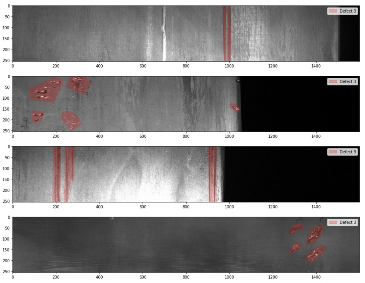
Example steel surfaces with manufacturing defects and segmentation masks overlaid.
As a rule of thumb increased variance in a data set necessitates more examples for robust learning, and this data set shows lots of variance. Given the relative spatial sparsity of defects, this data set also lends itself well to being formulated as a more coarse-grained image classification problem (”For a given region, is there a defect or not?”), which is generally understood to be a simpler task than segmentation. Therefore in order to have the best shot at both generating plausible synthetic data and understanding its impact, we opted to formulate a new classification task and analyze the impact of synthetic data on that, instead of considering the original segmentation problem.
The classification problem considers crops of the original data set. The crops were chosen according to some heuristics that were intended primarily to reduce the variance in size and position of defects, namely:
- Defect instances must fit entirely in the crop.
- Defect instances must be approximately centered in the crop.
- Crops must not overlap the edge of the image, or include any portion of the above mentioned dark regions.
- The crop dimensions were selected to include the majority of defects, excluding only the largest ones that were extraordinarily wide. (Smaller images ease the compute burden significantly.)
We also dropped three of the four original defect classes entirely, so the resulting task is a binary classification problem to identify whether a crop exhibits a defect or not. This remains an imbalanced problem with orders of magnitude more examples of non-defective crops than defective crops. By varying the number of defective and non-defective crops we consider, we can artificially construct either a perfectly balanced data set where the number of non-defective and defective crops are equal, or one that is higly imbalanced in favor of non-defective crops. This spectrum of data sets and the classification task defined on it will ultimately be the playground on which we evaluate the quality of our synthetic data generation models, but first we needed to convince ourselves that we could generate plausible synthetic data at all.
We also incorporated a subset of ImageNet, namely the same images of horses and zebras that were used in Zhu et al., “Unpaired Image-To-Image Translation Using Cycle-Consistent Adversarial Networks,” in order to qualitatively validate our implementation.
What is CycleGAN? Why use it for this problem?
A “vanilla” GAN is a set of two parameterized networks, typically called the generator and discriminator, that alternately seek to minimize and maximize some objective function with respect to their weights.10 CycleGAN consists of two “vanilla” GANs that learn mappings that are each other’s inverse, and this relationship is used to define a new cycle-consistency loss term that is minimized when this inverse relationship is learned perfectly. For example Zhu et al. learn a pair of such mappings that turn images of horses into zebras, as well as the opposite:
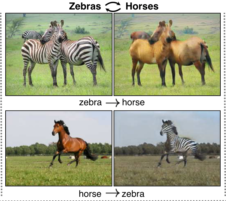
Image from Zhu et al.
The notion of cycle-consistency arises from the observation that if you turn an image of a horse into a zebra, then back to a horse, this round trip could plausibly yield the same exact horse image. The cycle-consitency loss measures the extent to which it does not.
This problem is intuitively appealing because horses and zebras already kinda look alike. As a human if you wanted to turn zebras into horses for some reason11 a “simple” procedure to do it could be to erase the zebra’s stripes with your magic eraser, then fill in the erased part with brownish colors. And that’s it. Horses and zebras tend to be in similar looking backgrounds, so we don’t have to change that to produce a plausible result. We know more or less what the ideal solution is, it just happens to be currently impossible to create a program that does it well without deep learning.
The steel defect classification problem we formulated is analogous. As a human, if you wanted to turn images of defect-free steel surfaces into images of defective steel surfaces, a “simple” procedure to do it would be to draw some pitting or scratches on top of the defect-free surface, if you knew what they looked like. And that’s it. Once again, we know more or less what the ideal solution is, it just happens to be currently impossible to create a program that does it well without deep learning.
Iteration 0
First I needed to “bootstrap” my implementation of CycleGAN. Supposing I wrote an implementation but found I couldn’t create plausible synthetic manufacturing defects, how would I determine whether the fault was in my implementation, or if we simply didn’t have enough data? I cannot possibly hope to disentangle these considerations by examining results on the manufacturing defect data set alone. A logical step then is to recreate some previously published result, so I chose to focus on the horse-to-zebra object transfiguration task (henceforth horse2zebra).
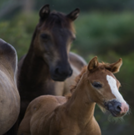
Sparing the details, my implementation strategy was to closely read Zhu et al. and carefully implement what is described in that paper. I expected to make mistakes at this point - there are so many moving parts that it would be a wonder if I didn’t. After training for 200 epochs, taking about 5 hours on the V100 GPU available to me, here’s one result:
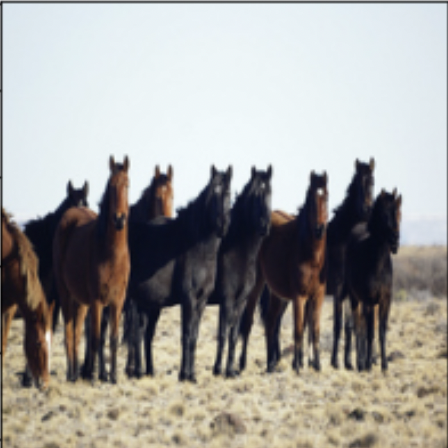
Left: source image of horses. Right: learned image of zebras.
Intriguing, but not very plausible.
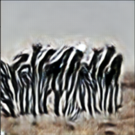
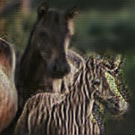
There is a generously open-source implementation of CycleGAN12 that had qualitatively far better results early in training:
Left: same source image of horses. Right: improved learned image of zebras.
The evaluation is summarized in the following matrix:
| …on my best horse2zebra result so far, on its own merits. | …on my best horse2zebra result so far, compared to reference implementation. | |
|---|---|---|
| Mike’s opinion… | Not plausible. | Obvious quality differences. |
You might ask, “Why don’t you use the open source implementation?” if you forgot that I was doing this for self-indulgent reasons.
Iteration 1
Of course after reviewing the paper I made a number of changes to my implementation to match what was described. Even after that, I found some notable differences between my implementation and the open source implementation, including that the open source implementation used a generator model with more layers. Additionally, Zhu et al. describe an identity loss term that I didn’t notice at first, but that has a significant impact on the results:
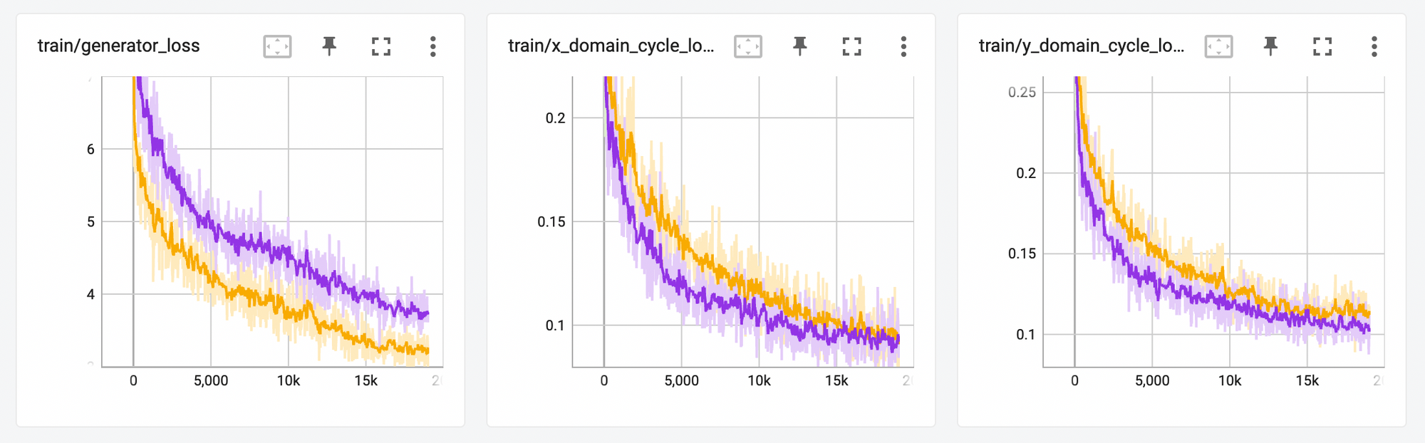
Left: overall generator loss. Middle, right: two cycle consistency loss terms.
The three graphs depict the overall generator loss (left) and two cycle consistency loss terms (middle and right). The purple line depicts a model trained with an identity loss term, and the orange without. Finally the darker lines are smoothed versions of the lighter lines - the losses oscillate rapidly during training, and smoothing can help identify coarse trends.
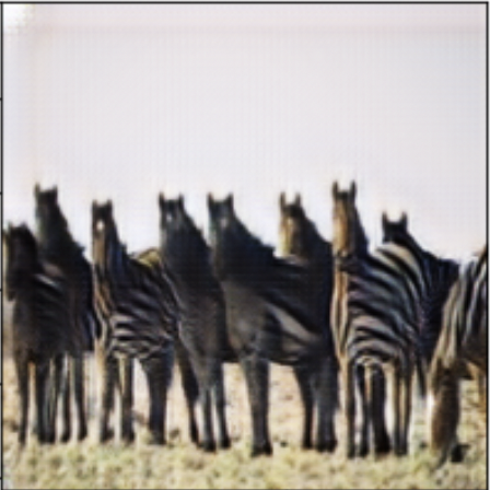
With identity loss included the overall generator loss is higher since we are adding a new nonnegative term, as depicted in the leftmost graph. Notably however, the introduction of the identity loss term has an additional effect of pushing the cycle consistency loss down, illustrated by the purple line trending lower than the orange in the middle and right graphs. Here’s an example source horse image and the resulting zebra from my horse2zebra model at this point:
The evaluation is summarized in the following matrix:
| …on my best horse2zebra result so far, on its own merits. | …on my best horse2zebra result so far, compared to reference implementation. | |
|---|---|---|
| Mike’s opinion… | Still not plausible, but a little bit improved from the previous iteration. | Obvious quality differences - severe distortion/noise around the horse in the foreground, and an unusual texture on the rest of the image. |
Note that I am not training these models to “completion” for two reason:
- Given that the loss oscillates so much, it was not clear to me that it would converge, which begs the question of what “training to completion” even means in this context. Zhu et al., for example, report training for a fixed number of epochs regardless of the loss achieved.
- The training times on the compute resources available to me could already be measured in hours. Before committing resources for a longer training protocol, I wanted to convince myself that I had eliminated any obvious errors.
Iteration 2
In the final horse2zebra iteration I did indeed discover some more discrepancies in my implementation compared to the description in Zhu et al. - I needed to change some hyperparameters and scale a loss term differently. Consider the following two sets of fake zebras:
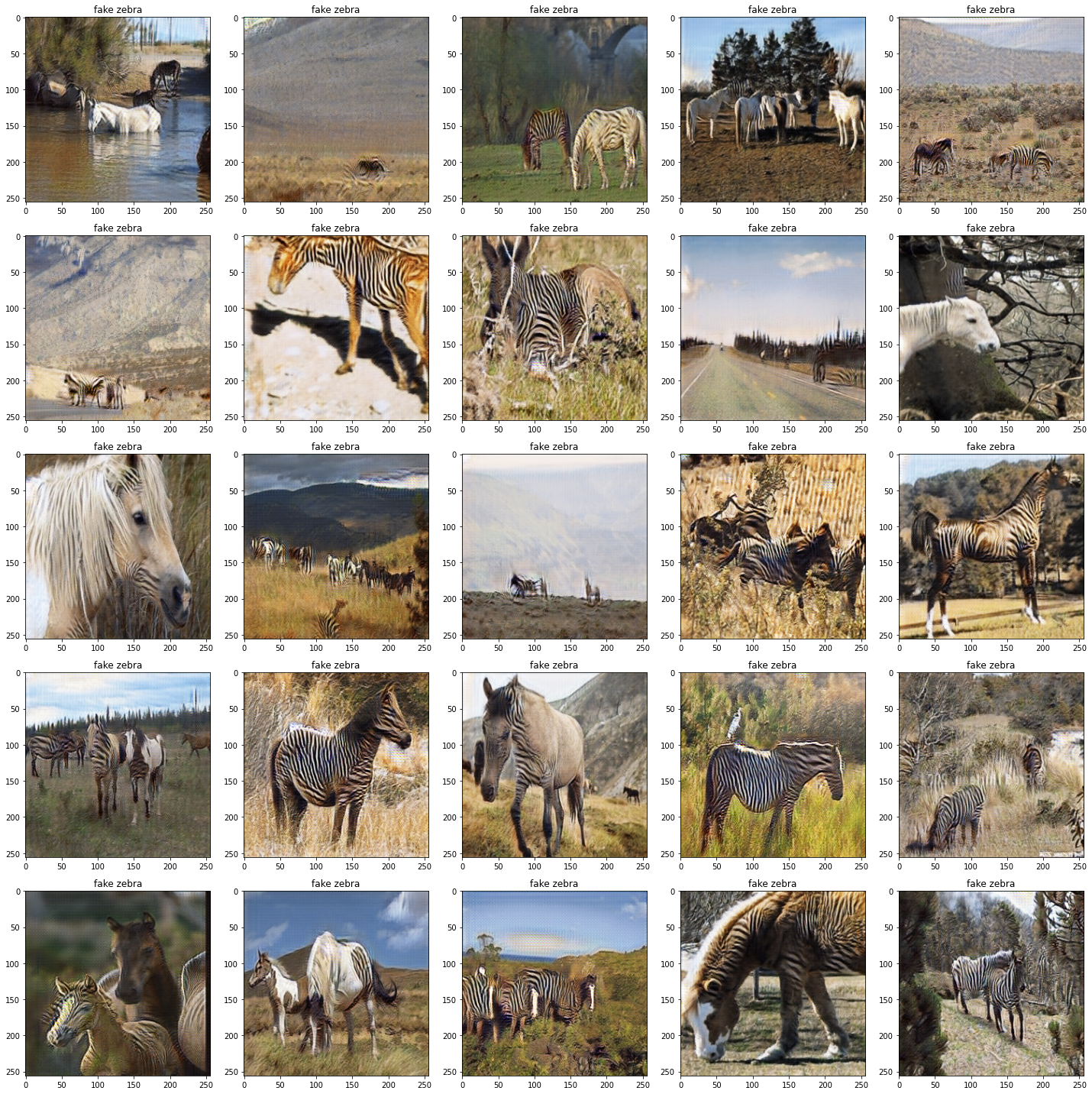
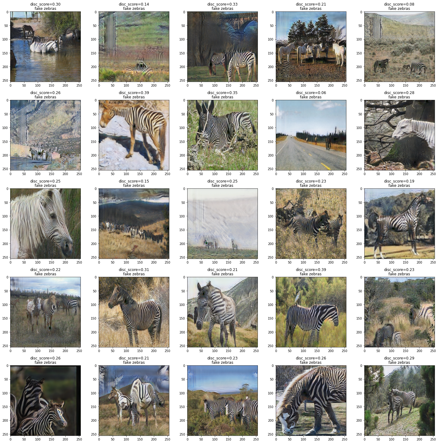
Two sets of fake zebras, generated by two different CycleGAN models. Click to see full-size versions.
One is generated from the reference implementation and the other from my implementation, trained for the same number of epochs. To my eye, they are qualitatively similar, and I wanted to conclude that my implementation was able to reproduce the published results. I polled my coworkers on which set of images they felt was more plausible in order to hedge against my personal bias. We all used different methodologies, including one “sophisticated point system.”
The evaluation is summarized in the following matrix:
| …on my best horse2zebra result so far, on its own merits. | …on my best horse2zebra result so far, compared to reference implementation. | |
|---|---|---|
| Mike’s opinion… | Plausible in several cases, however with obvious distortions in many cases. | Comparable. |
| Melanie’s opinion… | Right hand side is more plausible. | |
| Andrew’s opinion… | Right hand side is slightly more plausible. | |
| Juno’s opinion… | Zebra quality is comparable, but background quality is less plausible on the left hand side. |
Your bonus assignment is to pick out which set of images you think I generated and which set was generated with the reference implementation. Then select the following text to reveal the answer: the right hand side is my implementation and the left hand side is the reference implementation.
The only loose thread now is how to know when to stop training. Should I train for a fixed number of iterations, or stop if the the loss doesn’t decrease for a certain number of epochs? Or perhaps use some more sophisticated heuristic? In general for supervised learning one may stop training early once loss has converged, but that is not a reliable criterion when the loss oscillates rapidly as with CycleGAN. In fact my qualitatively best horse2zebra result is not from the model that achieved minimum loss, as one might expect - the model with minimum loss tended to have very distorted backgrounds. Heusel et al.13 show that under certain conditions Frechet Inception Distance (FID) will converge for GANs, and so I began to monitor FID during training, observing that it did indeed converge. However FID and loss did not achieve their minimums simultaneously, which complicated the analysis. I started to use FID convergence as a necessary but not sufficient condition for training to be “complete.”
Synthetic Manufacturing Defects
Now that we have a CycleGAN implementation we’re pleased with and a strategy for our training protocol, we turn back to our steel data set. On the left are real manufacturing defects, and the right are non-defective regions:
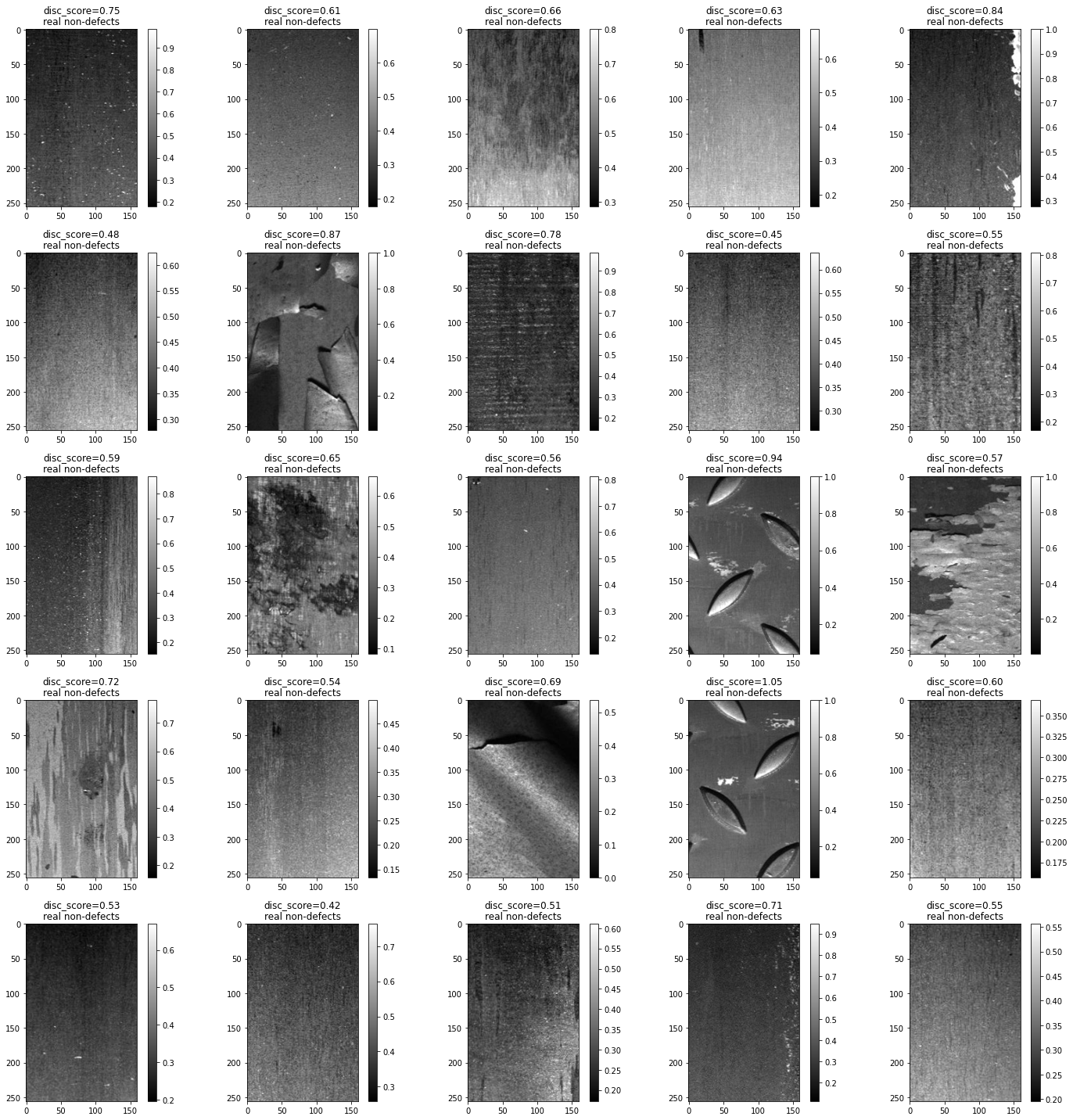
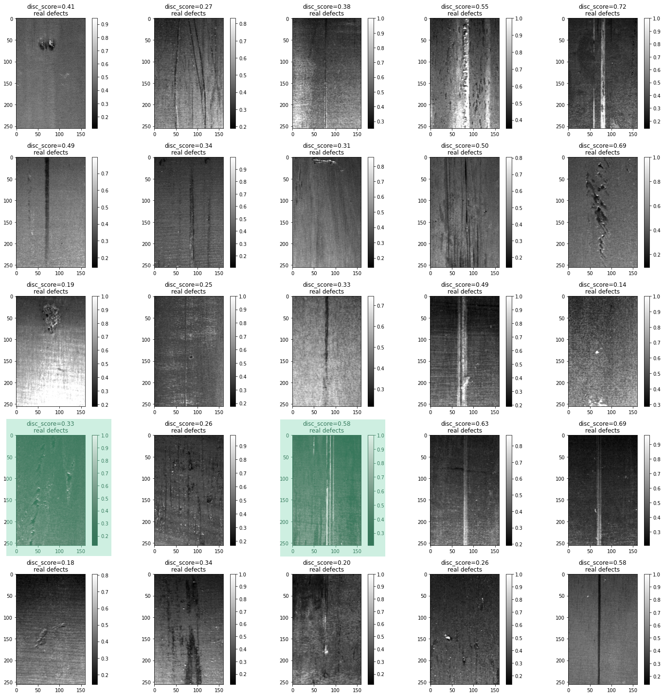
Left: non-defective crops. Right: defective crops. Click to view an enlarged version.
All the defects are of the same class according to the ground truth segmentation masks. Within this class though one can distinguish two different kinds of defects - for example compare columns 1 and 3 in row 4 (green overlay). The image in column 1 row 4 shows what look like small gouges that are relatively wide, and that appear in discontinuous streaks. The image in column 3 row 4 shows what looks like long parallel scratches that tend to span the whole y axis.
Now compare to synthetic defects from a model trained for 100 epochs:
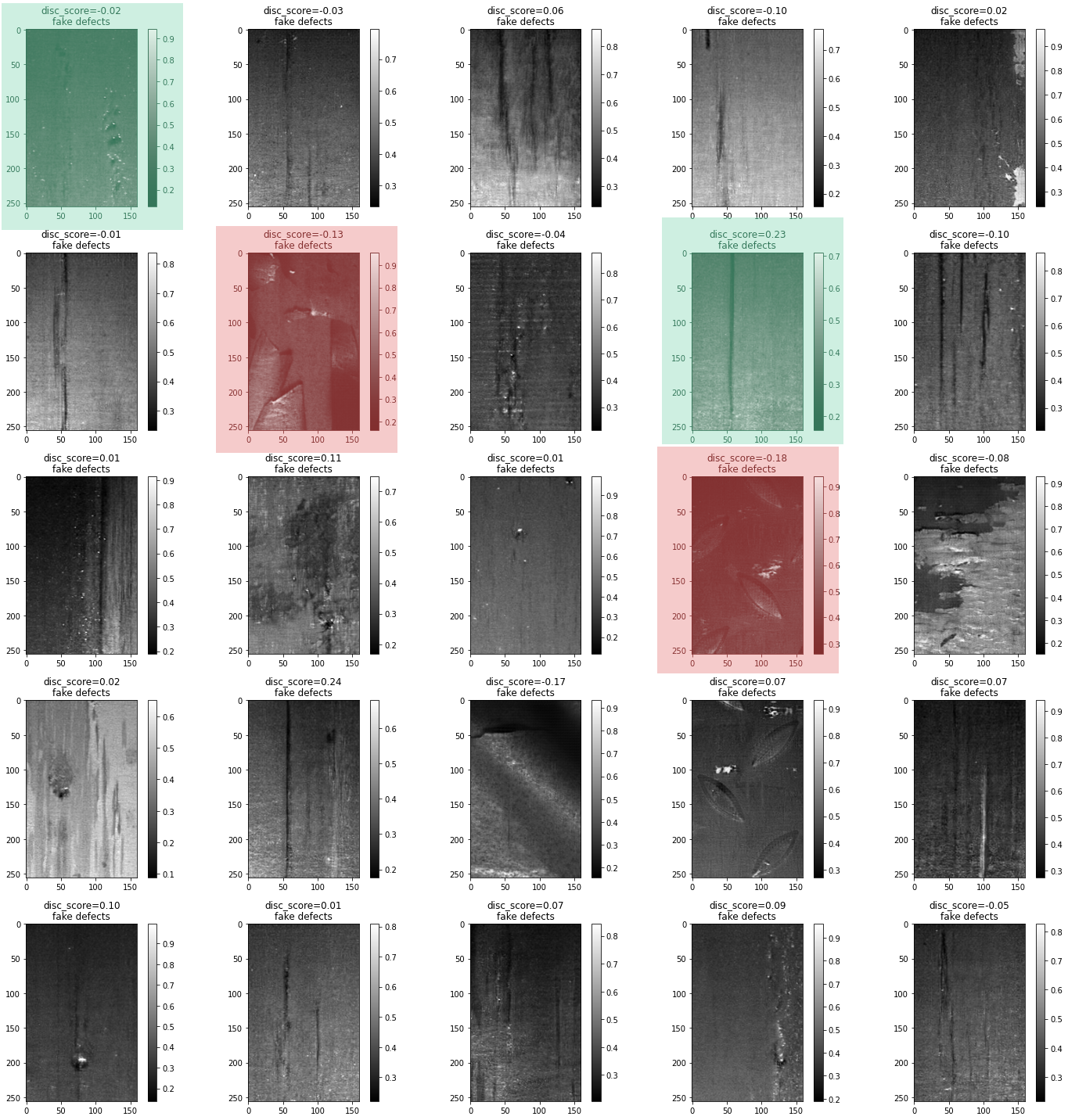
Not all the images are plausible - especially those derived from non-defective images with unusual textures or metal shavings in the crop (red overlays) - but many of them are to my eye, and both kinds of defects are exhibited (green overlays). Once again FID apparently converged but does not achieve its minimum simultaneously with the loss:
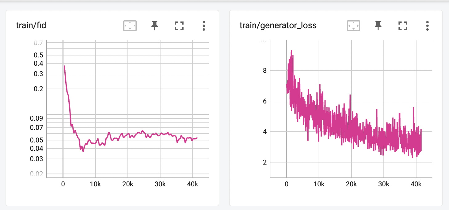
Huzzah! I’m calling this a success. While it certainly would be possible to pursue better results, qualitatively they’re pretty ok. Since this is only one part of an overarching research effort, we actually have a plan to evaluate the results quantitatively in the near future.
What comes next?
Ok, we satisfied ourselves that we can plausibly produce synthetic manufacturing defects, but so what? Given that we have an imbalanced (read: challenging) classification problem motivating this research effort, we’d obviously like to understand what impact incorporating synthetic data has on that task. We expect inferior performance on the minority class of defects, and so the basic recipe is to incorporate synthetic examples of the minority class and observe how it changes task performance by class. There are many dimensions of possible improvement to consider, including:
- Does incorporating synthetic data along with all available real data in training improve task performance? In other words, can we get more out of the data we collect by “simply” using it to generate synthetic data?
- Can we achieve comparable performance using a model that is trained on only a subset of the available real data, augmented with synthetic data? In other words, if we use synthetic data can we avoid collecting more real data in the first place, which is often a costly and challenging aspect to developing deep learning models?
- Assuming that incorporating synthetic data in training does improve task performance, one can also ask how much real data is needed to bootstrap the synthetic data generation model.
Look to a future post for results!
References
-
Zhu, Jun-Yan, Taesung Park, Phillip Isola, and Alexei A. Efros. “Unpaired Image-To-Image Translation Using Cycle-Consistent Adversarial Networks,” 2223–32, 2017. https://openaccess.thecvf.com/content_iccv_2017/html/Zhu_Unpaired_Image-To-Image_Translation_ICCV_2017_paper.html. ↩︎
-
Fang, Qiang, Clemente Ibarra-Castanedo, and Xavier Maldague. “Automatic Defects Segmentation and Identification by Deep Learning Algorithm with Pulsed Thermography: Synthetic and Experimental Data.” Big Data and Cognitive Computing 5, no. 1 (March 2021): 9. https://doi.org/10.3390/bdcc5010009. ↩︎
-
Park, Deokhwan, Joosoon Lee, Junseok Lee, and Kyoobin Lee. “Deep Learning Based Food Instance Segmentation Using Synthetic Data.” In 2021 18th International Conference on Ubiquitous Robots (UR), 499–505, 2021. https://doi.org/10.1109/UR52253.2021.9494704. ↩︎
-
Zhang, Zizhao, Lin Yang, and Yefeng Zheng. “Translating and Segmenting Multimodal Medical Volumes With Cycle- and Shape-Consistency Generative Adversarial Network,” 9242–51, 2018. https://openaccess.thecvf.com/content_cvpr_2018/html/Zhang_Translating_and_Segmenting_CVPR_2018_paper.html. ↩︎
-
Huo, Yuankai, Zhoubing Xu, Hyeonsoo Moon, Shunxing Bao, Albert Assad, Tamara K. Moyo, Michael R. Savona, Richard G. Abramson, and Bennett A. Landman. “SynSeg-Net: Synthetic Segmentation Without Target Modality Ground Truth.” IEEE Transactions on Medical Imaging 38, no. 4 (April 2019): 1016–25. https://doi.org/10.1109/TMI.2018.2876633. ↩︎
-
Mahmood, Faisal, Daniel Borders, Richard J. Chen, Gregory N. Mckay, Kevan J. Salimian, Alexander Baras, and Nicholas J. Durr. “Deep Adversarial Training for Multi-Organ Nuclei Segmentation in Histopathology Images.” IEEE Transactions on Medical Imaging 39, no. 11 (November 2020): 3257–67. https://doi.org/10.1109/TMI.2019.2927182. ↩︎
-
Writing from scratch is admittedly not always the best engineering decision to make, though. ↩︎
-
For example, 3D rendering technology achieves impressive results when informed by the physics of optics. See https://pbrt.org/ ↩︎
-
Employers take note: there is a place for fun and games at work. ↩︎
-
Goodfellow, Ian J., Jean Pouget-Abadie, Mehdi Mirza, Bing Xu, David Warde-Farley, Sherjil Ozair, Aaron Courville, and Yoshua Bengio. “Generative Adversarial Networks.” arXiv, June 10, 2014. https://doi.org/10.48550/arXiv.1406.2661. ↩︎
-
Drop me a line if you have a reason, I’d love to learn about it. ↩︎
-
Heusel, Martin, Hubert Ramsauer, Thomas Unterthiner, Bernhard Nessler, and Sepp Hochreiter. “GANs Trained by a Two Time-Scale Update Rule Converge to a Local Nash Equilibrium.” In Advances in Neural Information Processing Systems, Vol. 30. Curran Associates, Inc., 2017. https://papers.nips.cc/paper/2017/hash/8a1d694707eb0fefe65871369074926d-Abstract.html. ↩︎