Feb 24, 2016 · post
"Hello world" in Keras (or, Scikit-learn versus Keras)
This article is available as a notebook on Github. Please refer to that notebook for a more detailed discussion and code fixes and updates.
Despite all the recent excitement around deep learning, neural networks have a reputation among non-specialists as complicated to build and difficult to interpret.
And while interpretability remains an issue, there are now high-level neural network libraries that enable developers to quickly build neural network models without worrying about the numerical details of floating point operations and linear algebra.
This post compares keras with scikit-learn, the most popular, feature-complete classical machine learning library used by Python developers.
Keras is a high-level neural network library that wraps an API similar to scikit-learn around the Theano or TensorFlow backend. Scikit-learn has a simple, coherent API built around Estimator objects. It is carefully designed and is a good description of machine learning workflow with which many engineers are already comfortable.
Let’s get started by importing the libraries we’ll need: scikit-learn, keras and some plotting features.
>>> %matplotlib inline
>>> import seaborn as sns
>>> import numpy as np
>>> from sklearn.cross_validation import train_test_split
>>> from sklearn.linear_model import LogisticRegressionCV
>>> from keras.models import Sequential
>>> from keras.layers.core import Dense, Activation
>>> from keras.utils import np_utils
Iris data
The famous iris dataset is a great way of demonstrating the API of a machine learning framework. In some ways it’s the “Hello world” of machine learning.
The data is simple, and it’s possible to get high accuracy with an extremely simple classifier. Using a neural network here would be like using a sledghammer to crack a nut. But this is fine for us; we want to show the code required to get from data to working classifier, not the details of model design.
The iris dataset is built into many machine learning libraries. We like the copy in seaborn because it comes as a labelled dataframe that can be easily visualized. Let’s load it and look at the first 5 examples.
>>> iris = sns.load_dataset("iris")
>>> iris.head()
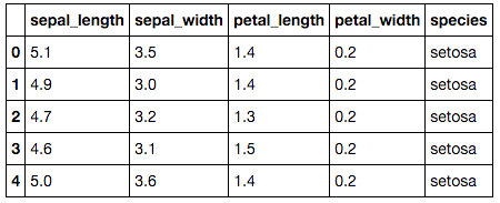
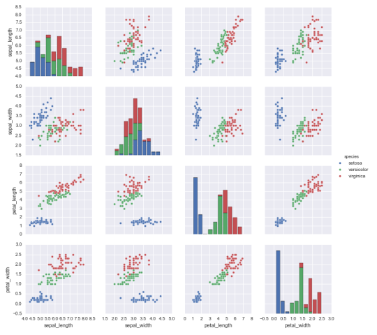
For each example (i.e., flower), there are five pieces of data. Four are standard measurements of the flower’s size (in centimeters), and the fifth is the species of iris. There are three species: setosa, verscicolor and virginica. Our job is to build a classifier that, given the two petal and two sepal measurements, can predict the species of an iris. Let’s do a quick visualization before we start model building (always a good idea!):
>>> sns.pairplot(iris, hue='species')
Munge and split the data for training and testing
First we need to pull the raw data out of the iris dataframe. We’ll hold the petal and sepal data in an array X and the species labels in a corresponding array y.
>>> X = iris.values[:, 0:4]
>>> y = iris.values[:, 4]
Now we split X and y in half. As is standard in supervised machine learning, we’ll train with half the data, and measure the performance of our model with the other half. This is simple to do by hand, but is built into scikit-learn as the train_test_split()function.
>>> train_X, test_X, train_y, test_y = train_test_split(X, y, train_size=0.5, random_state=0)
Train a scikit-learn classifier
We’ll train a logisitic regression classifier. Doing this, with built-in hyper-paramter cross validation, requires one line in scikit-learn. Like all scikit-learn Estimator objects, a LogisticRegressionCV classifier has a .fit() method that takes care of the gory numerical details of learning model parameters that best fit the training data. So that method is all we need to do:
>>> lr = LogisticRegressionCV()
>>> lr.fit(train_X, train_y)
Assess the classifier using accuracy
Now we can measure the fraction of of the test set the trained classifer classifies correctly (i.e., accuracy).
>>> pred_y = lr.predict(test_X)
>>> print("Test fraction correct (Accuracy) = {:.2f}".format(lr.score(test_X, test_y)))
# Test fraction correct (Accuracy) = 0.83
Now do something very similar with Keras
Scikit-learn makes building a classifier very simple:
- one line to instantiate the classifier
- one line to train it
- and one line to measure its performance
It’s only a little bit more complicated in keras.
First a bit of data-munging: scikit-learn’s classifiers accept string labels, e.g. "setosa". But keras requires that labels be one-hot-encoded. This means we need to convert data that looks like
setosa
versicolor
setosa
virginica
...
to a table that looks like
setosa versicolor virginica
     1          0         0
     0          1         0
     1          0         0
     0          0         1
There are lots of ways of doing this. We’ll use a keras utility and some numpy.
>>> def one_hot_encode_object_array(arr):
    '''One hot encode a numpy array of objects (e.g. strings)'''
    uniques, ids = np.unique(arr, return_inverse=True)
    return np_utils.to_categorical(ids, len(uniques))

>>> train_y_ohe = one_hot_encode_object_array(train_y)
>>> test_y_ohe = one_hot_encode_object_array(test_y)
Build the neural network model
Building the model is the only aspect of using keras that is substantially more code than in scikit-learn.
Keras is a neural network library. As such, while the number of features/classes in your data provide constraints, you can determine all other aspects of model structure. This means that instaniating the classifier requires more work than the one line required by scikit-learn.
In this case, we’ll build an extremely simple network: 4 features in the input layer (the four flower measurements), 3 classes in the ouput layer (corresponding to the 3 species), and 16 hidden units because (from the point of view of a GPU, 16 is a round number!)
>>> model = Sequential()
>>> model.add(Dense(16, input_shape=(4,)))
>>> model.add(Activation('sigmoid'))
>>> model.add(Dense(3))
>>> model.add(Activation('softmax'))
>>> model.compile(loss='categorical_crossentropy', optimizer='adam')
But now we’ve instantiated the keras model, we have an object whose API is almost identical to a classifier in scikit-learn. In particular, it has .fit() and .predict() methods. Let’s fit:
>>> model.fit(train_X, train_y_ohe, verbose=0, batch_size=1)
For basic use, the only syntactic API difference between a compiled keras model and a sklearn classifier is that keras’s equivalent of the sklearn .score() method is called .evaluate(). By default it returns whatever loss function you set when you compile the model, but we can ask it to return the accuracy too. In this case, the second number it returns is exactly what you’d get from .score() in sklearn.
>>> loss, accuracy = model.evaluate(test_X, test_y_ohe, show_accuracy=True, verbose=0)
>>> print("Test fraction correct (Accuracy) = {:.2f}".format(accuracy))

# Test fraction correct (Accuracy) = 0.99
As you can see, the test accuracy of the neural network model is better than that of the simple logistic regression classifier.
While reassuring, this misses the point: a neural network model is overkill for this problem. But note that using a batteries-included, high-level library like keras requires only marginally more code to build, train, and apply a neural network model than a traditional model.
What’s next
There’s a point where the high-level keras approach does not provide the flexibility needed to build a complex or novel neural network model, but fortunately most work won’t reach that level of complexity.
We built an extremely simple feed-forward network model. To learn more, have a look at this MNIST tutorial, which demonstrates a slighty more complex use case: the MNIST handwritten digits data. This data requires the complexity a neural network model can afford, with performance improved via a deeper model with some dropout (an approach to regularization in neural networks).
keras also has layers that allow you to build models with:
- convolutional neural networks, which give state-of-the-art results for computer vsion problems
- recurrent neural networks, which are particularly well suited to modelling language and other sequence data.
In fact, one key strength of neural networks (along with sheer predictive power) is their composability. Using a high-level library like keras, it only takes a few seconds of work to create a very different network. Models can be built up like legos. Sure, the computer then has to grind through training on a GPU, and that’s still relatively expensive. But while the computer slaves away, you get to have fun.
- Mike

