Aug 22, 2016 · whitepaper

Under the Hood of the Variational Autoencoder (in Prose and Code)

The Variational Autoencoder (VAE) neatly synthesizes unsupervised deep learning and variational Bayesian methods into one sleek package. In Part I of this series, we introduced the theory and intuition behind the VAE, an exciting development in machine learning for combined generative modeling and inference—“machines that imagine and reason.”

To recap: VAEs put a probabilistic spin on the basic autoencoder paradigm—treating their inputs, hidden representations, and reconstructed outputs as probabilistic random variables within a directed graphical model. With this Bayesian perspective, the encoder becomes a variational inference network, mapping observed inputs to (approximate) posterior distributions over latent space, and the decoder becomes a generative network, capable of mapping arbitrary latent coordinates back to distributions over the original data space.

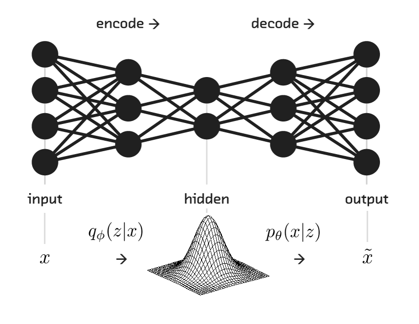
The beauty of this setup is that we can take a principled Bayesian approach toward building systems with a rich internal “mental model” of the observed world, all by training a single, cleverly-designed deep neural network.

These benefits derive from an enriched understanding of data as merely the tip of the iceberg—the observed result of an underlying causative probabilistic process.

The power of the resulting model is captured by Feynman’s famous chalkboard quote: “What I cannot create, I do not understand.” When trained on MNIST handwritten digits, our VAE model can parse the information spread thinly over the high-dimensional observed world of pixels, and condense the most meaningful features into a structured distribution over reduced latent dimensions.

Having recovered the latent manifold and assigned it a coordinate system, it becomes trivial to walk from one point to another along the manifold, creatively generating realistic digits all the while:

In this post, we’ll take a look under the hood at the math and technical details that allow us to optimize the VAE model we sketched in Part I.

Along the way, we’ll show how to implement a VAE in TensorFlow—a library for efficient numerical computation using data flow graphs, with key features like automatic differentiation and parallelizability (across clusters, CPUs, GPUs…and TPUs if you’re lucky). You can find (and tinker with!) the full implementation here, along with a couple pre-trained models.

Building the Model

Let’s dive into code (Python 3.4), starting with the necessary imports:

from functional import compose, partial import numpy as np import tensorflow as tf

<p>One perk of these models is their modularity—VAEs are naturally amenable to swapping in whatever encoder/decoder architecture is most fitting for the task at hand: <a href="https://arxiv.org/abs/1502.04623">recurrent</a> <a href="https://arxiv.org/abs/1511.06349">neural</a> <a href="https://arxiv.org/abs/1412.6581">networks</a>, <a href="https://arxiv.org/abs/1411.5928">convolutional</a> and <a href="https://arxiv.org/abs/1503.03167">deconvolutional</a> networks, etc.</p>
<p>For our purposes, we will model the relatively simple <a href="http://yann.lecun.com/exdb/mnist/">MNIST</a> dataset using densely-connected layers, wired symmetrically around the hidden code.</p>

```python
class Dense():
    """Fully-connected layer"""
    def __init__(self, scope="dense_layer", size=None, dropout=1.,
                 nonlinearity=tf.identity):
        # (str, int, (float | tf.Tensor), tf.op)
        assert size, "Must specify layer size (num nodes)"
        self.scope = scope
        self.size = size
        self.dropout = dropout # keep_prob
        self.nonlinearity = nonlinearity

    def __call__(self, x):
        """Dense layer currying, to apply layer to any input tensor `x`"""
        # tf.Tensor -&gt; tf.Tensor
        with tf.name_scope(self.scope):
            while True:
                try: # reuse weights if already initialized
                    return self.nonlinearity(tf.matmul(x, self.w) + self.b)
                except(AttributeError):
                    self.w, self.b = self.wbVars(x.get_shape()[1].value, self.size)
                    self.w = tf.nn.dropout(self.w, self.dropout)
    ...

We can initialize a Dense layer with our choice of nonlinearity for the layer nodes (i.e. neural network units that apply a nonlinear activation function to a linear combination of their inputs, as per line 18).

We’ll use ELUs (Exponential Linear Units), a recent advance in building nodes that learn quickly by avoiding the problem of vanishing gradients. We wrap up the class with a helper function (Dense.wbVars) for compatible random initialization of weights and biases, to further accelerate learning.

In TensorFlow, neural networks are defined as numerical computation graphs. We will build the graph using partial function composition of sequential layers, which is amenable to an arbitrary number of hidden layers.

i.e. composed = composeAll([f, g, h])
     composed(x) # == f(g(h(x)))
"""
# adapted from https://docs.python.org/3.1/howto/functional.html
return partial(functools.reduce, compose)(*args)

<p>Now that we’ve defined our model primitives, we can tackle the VAE itself.</p>
<p>Keep in mind: the TensorFlow computational graph is cleanly divorced from the numerical computations themselves. In other words, a <code>tf.Graph</code> wireframes the underlying skeleton of the model, upon which we may hang values only within the context of a <code>tf.Session</code>.</p>
<p>Below, we initialize class <code>VAE</code> and activate a session for future convenience (so we can initialize and evaluate tensors within a single session, e.g. to persist weights and biases across rounds of training).</p>
<p>Here are some relevant snippets, cobbled together from the <a href="https://github.com/fastforwardlabs/vae-tf/blob/master/vae.py">full source code</a>:</p>

```python
class VAE():
    """Variational Autoencoder

    see: Kingma &amp; Welling - Auto-Encoding Variational Bayes
    (https://arxiv.org/abs/1312.6114)
    """
    DEFAULTS = {
        "batch_size": 128,
        "learning_rate": 1E-3,
        "dropout": 1., # keep_prob
        "lambda_l2_reg": 0.,
        "nonlinearity": tf.nn.elu,
        "squashing": tf.nn.sigmoid
    }
    RESTORE_KEY = "to_restore"

    def __init__(self, architecture, d_hyperparams={}, meta_graph=None,
                 save_graph_def=True, log_dir="./log"):
        """(Re)build a symmetric VAE model with given:

         * architecture (list of nodes per encoder layer); e.g.
           [1000, 500, 250, 10] specifies a VAE with 1000-D inputs, 10-D latents,
           &amp; end-to-end architecture [1000, 500, 250, 10, 250, 500, 1000]

         * hyperparameters (optional dictionary of updates to `DEFAULTS`)
        """
        self.architecture = architecture
        self.__dict__.update(VAE.DEFAULTS, **d_hyperparams)
        self.sesh = tf.Session()

        if not meta_graph: # new model
            handles = self._buildGraph()
            ...
            self.sesh.run(tf.initialize_all_variables())

Assuming that we are building a model from scratch (rather than restoring a saved meta_graph), the key initialization step is the call to VAE._buildGraph (line 32). This internal method constructs nodes representing the placeholders and operations through which the data will flow—before any data is actually piped in.

Finally, we unpack the iterable handles (populated by _buildGraph) into convenient class attributes—pointers not to numerical values, but rather to nodes in the graph:

How are these nodes defined? The _buildGraph method encapsulates the core of the VAE model framework—starting with the encoder/inference network:

    # encoding / "recognition": q(z|x)
    encoding = [Dense("encoding", hidden_size, dropout, self.nonlinearity)
                # hidden layers reversed for function composition: outer -> inner
                for hidden_size in reversed(self.architecture[1:-1])]
    h_encoded = composeAll(encoding)(x_in)

    # latent distribution parameterized by hidden encoding
    # z ~ N(z_mean, np.exp(z_log_sigma)**2)
    z_mean = Dense("z_mean", self.architecture[-1], dropout)(h_encoded)
    z_log_sigma = Dense("z_log_sigma", self.architecture[-1], dropout)(h_encoded)

<p>Here, we build a pipe from <code>x_in</code> (an empty placeholder for input data <span class="math inline">\(x\)</span>), through the sequential hidden encoding, to the corresponding distribution over latent space—the variational approximate posterior, or hidden representation, <span class="math inline">\(z \sim q_\phi(z|x)\)</span>.</p>
<p>As observed in lines <code>14</code> - <code>15</code>, latent <span class="math inline">\(z\)</span> is distributed as a multivariate <a href="http://www.ncbi.nlm.nih.gov/pmc/articles/PMC2465539/figure/fig1/">normal</a> with mean <span class="math inline">\(\mu\)</span> and diagonal covariance values <span class="math inline">\(\sigma^2\)</span> (the square of the “sigma” in <code>z_log_sigma</code>) directly parameterized by the encoder: <span class="math inline">\(\mathcal{N}(\mu, \sigma^2I)\)</span>. In other words, we set out to “explain” highly complex observations as the consequence of an unobserved collection of simplified latent variables, i.e. independent Gaussians. (This is dictated by our choice of a conjugate spherical Gaussian prior over <span class="math inline">\(z\)</span>—see <a href="http://blog.fastforwardlabs.com/2016/08/12/introducing-variational-autoencoders-in-prose-and.html">Part I</a>.)</p>
<p>Next, we sample from this latent distribution (in practice, <a href="https://arxiv.org/abs/1312.6114">one draw is enough</a> given sufficient minibatch size, i.e. &gt;100). This method involves a trick—can you figure out why?—that we will explore in more detail later.</p>
```python
        z = self.sampleGaussian(z_mean, z_log_sigma)

The sampled \(z\) is then passed to the decoder/generative network, which symmetrically builds back out to generate the conditional distribution over input space, reconstruction \(\tilde{x} \sim p_\theta(x|z)\).

        # decoding / "generative": p(x|z)
        decoding = [Dense("decoding", hidden_size, dropout, self.nonlinearity)
                    for hidden_size in self.architecture[1:-1]] # assumes symmetry
        # final reconstruction: restore original dims, squash outputs [0, 1]
        decoding.insert(0, Dense( # prepend as outermost function
            "reconstruction", self.architecture[0], dropout, self.squashing))
        x_reconstructed = tf.identity(composeAll(decoding)(z), name="x_reconstructed")

Alternately, we add a placeholder to directly feed arbitrary values of \(z\) to the generative network (to fabricate realistic outputs—no input data necessary!):

        # ops to directly explore latent space
        # defaults to prior z ~ N(0, I)
        z_ = tf.placeholder_with_default(tf.random_normal([1, self.architecture[-1]]),
                                         shape=[None, self.architecture[-1]],
                                         name="latent_in")
        x_reconstructed_ = composeAll(decoding)(z_)

TensorFlow automatically flows data through the appropriate subgraph, based on the nodes that we fetch and feed with the tf.Session.run method. Defining the encoder, decoder, and end-to-end VAE is then trivial (see linked code).

We’ll finish the VAE._buildGraph method later in the post, as we walk through the nuances of the model.

The Reparameterization Trick

In order to estimate the latent representation \(z\) for a given observation \(x\), we want to sample from the approximate posterior \(q_\phi(z|x)\) according to the distribution defined by the encoder.

However, model training by gradient descent requires that our model be differentiable with respect to its learned parameters (which is how we propagate the gradients). This presupposes that the model is deterministic—i.e. a given input always returns the same output for a fixed set of parameters, so the only source of stochasticity are the inputs. Incorporating a probabilistic “sampling” node would make the model itself stochastic!

Instead, we inject randomness into the model by introducing input from an auxiliary random variable: \(\epsilon \sim p(\epsilon)\).

For our purposes, rather than sampling \(z\) directly from \(q_\phi(z|x) \sim \mathcal{N}(\mu, \sigma^2I)\), we generate Gaussian noise \(\epsilon \sim \mathcal{N}(0, I)\) and compute \[z = \mu + \sigma \odot \epsilon\] (where \(\odot\) is the element-wise product). In code:

    def sampleGaussian(self, mu, log_sigma):
        """Draw sample from Gaussian with given shape, subject to random noise epsilon"""
        with tf.name_scope("sample_gaussian"):
            # reparameterization trick
            epsilon = tf.random_normal(tf.shape(log_sigma), name="epsilon")
            return mu + epsilon * tf.exp(log_sigma) # N(mu, sigma**2)

By “reparameterizing” this step, inference and generation become entirely differentiable and hence, learnable.

Cost Function

Now, in order to optimize the model, we need a metric for how well its parameters capture the true data-generating and latent distributions. That is, how likely is observation \(x\) under the joint distribution \(p(x, z)\)?

Recall that we represent the global encoder and decoder parameters (i.e. neural network weights and biases) as \(\phi\) and \(\theta\), respectively.

In other words, we want to simultaneously tune these complementary parameters such that we maximize \(log(p(x|\phi, \theta))\)—the log-likelihood across all datapoints \(x\) under the current model settings, after marginalizing out the latent variables \(z\). This term is also known as the model evidence.

We can express this marginal likelihood as the sum of what we’ll call the variational or evidence lower bound \(\mathcal{L}\) and the Kullback-Leibler (KL) divergence \(\mathcal{D}_{KL}\) between the approximate and true latent posteriors: \[ log(p(x)) = \mathcal{L}(\phi, \theta; x) + \mathcal{D}_{KL}(q_\phi(z|x) || p_\theta(z|x)) \]

Here, the KL divergence can be (fuzzily!) intuited as a metric for the misfit of the approximate posterior \(q_\phi\). We’ll delve into this further in a moment, but for now the important thing is that it is non-negative by definition; consequently, the first term acts as a lower bound on the total. So, we maximize the lower bound \(\mathcal{L}\) as a (computationally-tractable) proxy for the total marginal likelihood of the data under the model. (And the better our approximate posterior, the tighter the gap between the lower bound and the total model evidence.)

With some mathematical wrangling, we can decompose \(\mathcal{L}\) into the following objective function: \[ \mathcal{L}(\phi, \theta; x) = \mathbb{E}_{z \sim q_\phi(z|x)}[log(p_\theta(x|z))] - \mathcal{D}_{KL}(q_\phi(z|x) || p_\theta(z)) \] (Phrased as a cost, we optimize the model by minimizing \({-\mathcal{L}}\).)

Here, the perhaps unfriendly-looking first term is, in fact, familiar! It’s the probability density of generated output \(\tilde{x}\) given the inferred latent distribution over \(z\)—i.e. the (negative) expected reconstruction error. This loss term is intrinsic to perhaps every autoencoder: how accurately does the output replicate the input?

Choosing an appropriate metric for image resemblance is hard (but that’s another story). We’ll use the binary cross-entropy, which is commonly used for data like MNIST that can be modeled as Bernoulli trials. Expressed as a static method of the VAE class:

    @staticmethod
    def crossEntropy(obs, actual, offset=1e-7):
        """Binary cross-entropy, per training example"""
        # (tf.Tensor, tf.Tensor, float) -> tf.Tensor
        with tf.name_scope("cross_entropy"):
            # bound by clipping to avoid nan
            obs_ = tf.clip_by_value(obs, offset, 1 - offset)
            return -tf.reduce_sum(actual * tf.log(obs_) +
                                  (1 - actual) * tf.log(1 - obs_), 1)

The second term in the objective is the KL divergence of the prior \(p\) from the (approximate) posterior \(q\) over the latent space. We’ll approach this conceptually, then mathematically.

The KL divergence \(\mathcal{D}_{KL}(q||p)\) is defined as the relative entropy between probability density functions \(q\) and \(p\). In information theory, entropy represents information content (measured in nats), so \(\mathcal{D}_{KL}\) quantifies the information gained by revising the candidate prior \(p\) to match some “ground truth” \(q\).

In a related vein, the KL divergence between posterior and prior beliefs (i.e. distributions) can be conceived as a measure of “surprise”: the extent to which the model must update its “worldview” (parameters) to accomodate new observations.

(Note that the formula is asymmetric—i.e. \(\mathcal{D}_{KL}(q||p) \neq \mathcal{D}_{KL}(p||q)\)—with implications for its use in generative models. This is also why it is not a true metric.)

By inducing the learned approximation \(q_\phi(z|x)\) (the encoder) to match the continuous imposed prior \(p(z)\), the KL term encourages robustness to small perturbations along the latent manifold, enabling smooth interpolation within and between classes (e.g. MNIST digits). This reduces “spottiness” in the latent space that is often observed in autoencoders without such regularization.

Mathematical bonus: we can strategically choose certain conjugate priors over \(z\) that let us analytically integrate the KL divergence, yielding a closed-form equation. This is true of the spherical Gaussian we chose, such that \[ {-\mathcal{D}}_{KL}(q_\phi(z|x) || p_\theta(z)) = \frac{1} 2 \sum{(1 + log(\sigma^2) - \mu^2 - \sigma^2)} \] (summed over the latent dimensions). In TensorFlow, that looks like this:

    @staticmethod
    def kullbackLeibler(mu, log_sigma):
        """(Gaussian) Kullback-Leibler divergence KL(q||p), per training example"""
        # (tf.Tensor, tf.Tensor) -> tf.Tensor
        with tf.name_scope("KL_divergence"):
            # = -0.5 * (1 + log(sigma**2) - mu**2 - sigma**2)
            return -0.5 * tf.reduce_sum(1 + 2 * log_sigma - mu**2 -
                                        tf.exp(2 * log_sigma), 1)

Together, these complementary loss terms capture the trade-off between expressivity and concision, between data complexity and simplicity of the prior. Reconstruction loss pushes the model toward perfectionist tendencies, while KL loss (along with the addition of auxiliary noise) encourages it to explore sensibly.

To elaborate (building on the VAE._buildGraph method started above):

        # reconstruction loss: mismatch b/w x & x_reconstructed
        # binary cross-entropy -- assumes p(x) & p(x|z) are iid Bernoullis
        rec_loss = VAE.crossEntropy(x_reconstructed, x_in)

        # Kullback-Leibler divergence: mismatch b/w approximate posterior & imposed prior
        # KL[q(z|x) || p(z)]
        kl_loss = VAE.kullbackLeibler(z_mean, z_log_sigma)

        # average over minibatch
        cost = tf.reduce_mean(rec_loss + kl_loss, name="cost")

Beyond its concise elegance and solid grounding in Bayesian theory, the cost function lends itself well to intuitive metaphor:

Information theory-wise, the VAE is a terse game of Telephone, with the aim of finding the minimum description length to convey the input from end to end. Here, reconstruction loss is the information “lost in translation,” while KL loss captures how overly “wordy” the model must be to convey the message through an unpredictable medium (hidden code imperfectly optimized for the input data).

Or, framing the VAE as a lossy compression algorithm, reconstruction loss accounts for the fidelity of (de)compression while KL loss penalizes the model for using a sub-optimal compression scheme.

Training

At last, our VAE cost function in hand (after factoring in optional \(\ell_2\)-regularization), we finish VAE._buildGraph with optimization nodes to be evaluated at each step of SGD (with the Adam optimizer)…

        # optimization
        global_step = tf.Variable(0, trainable=False)
        with tf.name_scope("Adam_optimizer"):
            optimizer = tf.train.AdamOptimizer(self.learning_rate)
            tvars = tf.trainable_variables()
            grads_and_vars = optimizer.compute_gradients(cost, tvars)
            clipped = [(tf.clip_by_value(grad, -5, 5), tvar) # gradient clipping
                    for grad, tvar in grads_and_vars]
            train_op = optimizer.apply_gradients(clipped, global_step=global_step,
                                                 name="minimize_cost") # back-prop

…and return all of the nodes we want to access in the future to the VAE.__init__ method where buildGraph was called.

        return (x_in, dropout, z_mean, z_log_sigma, x_reconstructed,
                z_, x_reconstructed_, cost, global_step, train_op)

Using SGD to optimize the function parameters of the inference and generative networks simultaneously is called Stochastic Gradient Variational Bayes.

This is where TensorFlow really shines: all of the gradient backpropagation and parameter updates are performed via automatic differentation, and abstracted away from the researcher in the train_op (essentially) one-liner on line 48.

Model training (with optional cross-validation) is then as simple as feeding minibatches from dataset X to the x_in placeholder and evaluating (“fetching”) the train_op. Here are some relevant chunks, excerpted from the full class method:

    def train(self, X, max_iter=np.inf, max_epochs=np.inf, cross_validate=True,
              verbose=True, save=False, outdir="./out", plots_outdir="./png"):
        try:
            err_train = 0
            now = datetime.now().isoformat()[11:]
            print("------- Training begin: {} -------\n".format(now))

            while True:
                x, _ = X.train.next_batch(self.batch_size)
                feed_dict = {self.x_in: x, self.dropout_: self.dropout}
                fetches = [self.x_reconstructed, self.cost, self.global_step, self.train_op]
                x_reconstructed, cost, i, _ = self.sesh.run(fetches, feed_dict)

                err_train += cost

                if i%1000 == 0 and verbose:
                    print("round {} --> avg cost: ".format(i), err_train / i)

                if i >= max_iter or X.train.epochs_completed >= max_epochs:
                    print("final avg cost (@ step {} = epoch {}): {}".format(
                        i, X.train.epochs_completed, err_train / i))
                    now = datetime.now().isoformat()[11:]
                    print("------- Training end: {} -------\n".format(now))
                    break

Helpfully, TensorFlow comes with a built-in visualization dashboard. Here’s the computational graph for an end-to-end VAE with two hidden encoder/decoder layers (that’s what all the tf.name_scope-ing was for):

Wrapping Up

The future of deep latent models lies in models that can reason about the world—“understanding” complex observations, transforming them into meaningful internal representations, and even leveraging these representations to make decisions—all while coping with scarce data, and in semisupervised or unsupervised settings. VAEs are an important step toward this future, demonstrating the power of new ways of thinking that result from unifying variational Bayesian methods and deep learning.

We now understand how these fields come together to make the VAE possible, through a theoretically-sound objective function that balances accuracy (reconstruction loss) with variational regularization (KL loss), and efficient optimization of the fully differentiable model thanks to the reparameterization trick.

We’ll wrap up for now with one more way of visualizing the condensed information encapsulated in VAE latent space.

Previously, we showed the correspondence between the inference and generative networks by plotting the encoder and decoder perspectives of the latent space in the same 2-D coordinate system. For the decoder perspective, this meant feeding linearly spaced latent coordinates to the generative network and plotting their corresponding outputs.

To get an undistorted sense of the full latent manifold, we can sample and decode latent space coordinates proportionally to the model’s distribution over latent space. In other words—thanks to variational regularization provided by the KL loss!—we simply sample relative to our chosen prior distribution over \(z\). In our case, this means sampling linearly spaced percentiles from the inverse CDF of a spherical Gaussian.¹

Once again, evolving over (logarithmic) time:

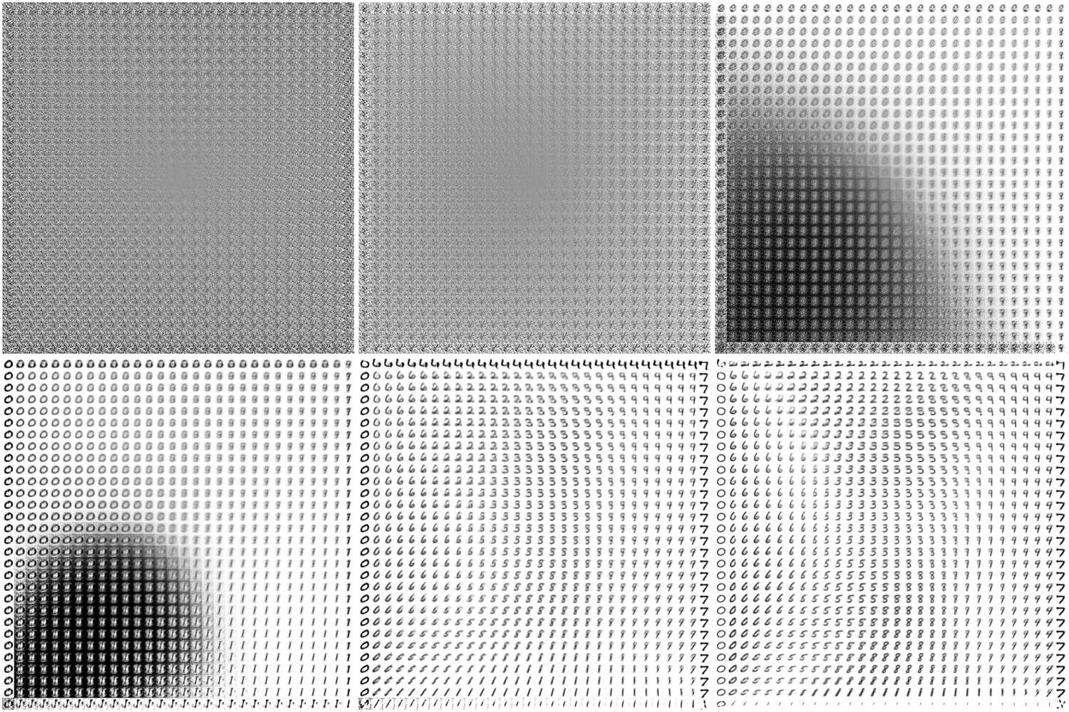
Interestingly, we can see that the slim tails of the distribution (edges of the frame) are not well-formed. Presumably, this results from few observed inputs being mapped to latent posteriors with significant density in these regions.

Here are a few resulting constellations (from a single model):

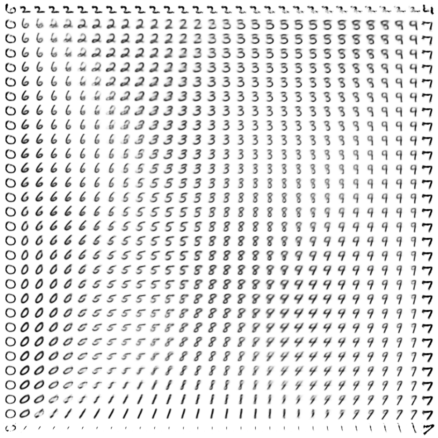
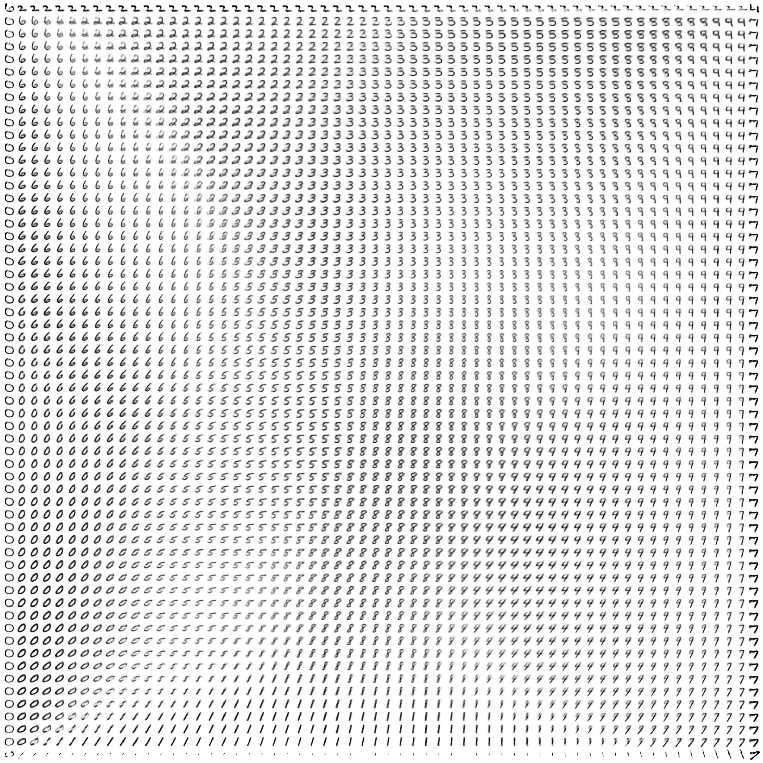
Theoretically, we could subdivide the latent space into infinitely many points (limited in practice only by the computer’s floating point precision), and let the generative network dream up infinite constellations of creative variations on MNIST.

That’s enough digits for now! Keep your eyes out for the next installment, where we’ll tinker with the vanilla VAE model in the context of a new dataset.

– Miriam

---

1. Thanks Kyle McDonald (@kcimc) and Tom White (@dribnet) for noting this!↩