Aug 12, 2016 · whitepaper
Introducing Variational Autoencoders (in Prose and Code)
Effective machine learning means building expressive models that sift out signal from noise—that simplify the complexity of real-world data, yet accurately intuit and capture its subtle underlying patterns.
Whatever the downstream application, a primary challenge often boils down to this: How do we represent, or even synthesize, complex data in the context of a tractable model?
This challenge is compounded when working in a limited data setting—especially when samples are in the form of richly-structured, high-dimensional observations like natural images, audio waveforms, or gene expression data.
Cue the Variational Autoencoder, a fascinating development in unsupervised machine learning that marries probabilistic Bayesian inference with deep learning.
Benefiting from advances in both research communities, the Variational Autoencoder addresses these challenges by leveraging innovative deep learning techniques grounded in a solid Bayesian theoretical framework…and can be explained through mesmerizing GIFs:

(Read on, and all will become clear…)
Intro
Traditional autoencoders are models (usually multilayer artificial neural networks) designed to output a reconstruction of their input. Specifically, autoencoders sequentially deconstruct input data into hidden representations, then use these representations to sequentially reconstruct outputs that resemble the originals. Fittingly, this process of teasing out a mapping from input to hidden representation is called representation learning.
The appeal of this setup is that the model learns its own definition of a “meaningful” representation based only on the data—no human-derived heuristics or labels! This approach stands in contrast to the majority of deep learning systems in production today, which rely on expensive-to-obtain labeled data (“This image is a kitten; this image is a panda.”). Alternatives to such supervised learning frameworks provide a way to benefit from a world brimming with valuable raw data.

Though trained holistically, autoencoders are often built for the part instead of the whole: researchers might exploit the data-to-representation mapping for semantic embeddings, or the representation-to-output mapping for extraordinarily complex generative modeling
But an autoencoder with unlimited capacity is doomed to the role of a wonky, computationally-expensive Xerox machine. To ensure that the transformations to or from the hidden representation are useful, we impose some type of regularization or constraint. As a tradeoff for some loss in fidelity, such impositions push the model to distill the most salient features from a cacophonous real-world dataset.
Variational Autoencoders (VAEs) incorporate regularization by explicitly learning the joint distribution over data and a set of latent variables that is most compatible with observed datapoints and some designated prior distribution over latent space. The prior informs the model by shaping the corresponding posterior, conditioned on a given observation, into a regularized distribution over latent space (the coordinate system spanned by the hidden representation).
As a result, VAEs are an excellent tool for manifold learning—recovering the “true” manifold in lower-dimensional space along which the observed data lives with high probability mass—and generative modeling of complex datasets like images, text, and audio—conjuring up brand new examples, consistent with the observed training set, that do not exist in nature.
Building on other informative posts, this is the first installment of a guide to Variational Autoencoders: the lovechild of Bayesian inference and unsupervised deep learning.
In this post, we’ll sketch out the model and provide an intuitive context for the math- and code-flavored follow-up. In Post II, we’ll walk through a technical implementation of a VAE (in TensorFlow and Python 3). In Post III, we’ll venture beyond the popular MNIST dataset using a twist on the vanilla VAE.
The Variational Autoencoder Setup
An end-to-end autoencoder (input to reconstructed input) can be split into two complementary networks: an encoder and a decoder. The encoder maps input \(x\) to a latent representation, or so-called hidden code, \(z\). The decoder maps the hidden code to a reconstructed input value \(\tilde x\).
Whereas a vanilla autoencoder is deterministic, a Variational Autoencoder is stochastic—a mashup of:
- a probabilistic encoder \(q_\phi(z|x)\), approximating the true (but intractable) posterior distribution \(p(z|x)\), and
- a generative decoder \(p_\theta(x|z)\), which notably does not rely on any particular input \(x\).
Both the encoder and decoder are artificial neural networks (i.e. hierarchical, highly nonlinear functions) with tunable parameters \(\phi\) and \(\theta\), respectively.
Learning these conditional distributions is facilitated by enforcing a plausible mathematically-convenient prior over the latent variables, generally a standard spherical Gaussian: \(z \sim \mathcal{N}(0, I)\).
Given this conjugate prior, the encoder’s job is to supply the mean and variance of the Gaussian posterior over each latent space dimension corresponding to a given input. Latent \(z\) is sampled from this distribution, then passed to the decoder to be transformed back into a distribution over the original data space.
In other words, a VAE represents a directed probabilistic graphical model, in which approximate inference is performed by the encoder and optimized alongside an easy-to-sample generative decoder. For this reason, these complementary halves are also known as the inference (or recognition) network and the generative network. By reformulating this graphical model as a differentiable neural net with a single, pithy cost function (derived from the variational lower bound), the whole package can be trained by stochastic gradient descent (SGD) thanks to the “amusing” universe we live in.
Bayes, Meet Neural Networks
In fact, many developments in deep learning research can also be understood through a probabilistic, or Bayesian, lens. Some of these analogies are more theoretical, whereas others share a parallel mathematical interpretation. For example, \(\ell_2\)-regularization can be viewed as imposing a Gaussian prior over neural network weights, and reinforcement learning can be formalized through variational inference.
VAEs exemplify a case where this relationship is made explicit and elegant, and variational Bayesian inference is the guiding principle shaping the model’s cost function and instrinsic architecture.
Why does this setup make sense?
In the Bayesian worldview, datapoints are observations drawn from some data-generating distribution: (observed) variable \(x \sim p(x)\). So, the MNIST dataset of handwritten digits describes a random variable with an intricate set of dependencies among all 28*28 pixels. Each MNIST image offers a glimpse into one arrangement of 784 pixel values with high probability—whereas a 28*28 block of white noise, or the Jolly Roger, (theoretically) occupy low probability mass under the distribution.

It would be a headache to model the conditional dependencies in 784-dimensional pixel space. Instead, we make the simplifying assumption that the distribution over these observed variables is the consequence of a distribution over some set of hidden variables: \(z \sim p(z)\). Intuitively, this paradigm is analogous to how scientists study the natural world, by working backwards from observed phenomena to recover the unifying hidden laws that govern them. In the case of MNIST, these latent variables could represent concepts like number identity and tiltedness, whereas more complex natural images like the Frey faces could have latent dimensions for facial expression and azimuth.
Inference is the process of disentangling these rich real-world dependencies into simplified latent dependencies, by predicting \(p(z|x) -\) the distribution over one set of variables (the latent variables) conditioned on another variable (the observed data). (This is where Bayes’ theorem enters the picture.)
With this Bayesian frame-of-mind, training a generative model is the same as learning the joint distribution over the data and latent variables: \(p(x, z)\). This approach lends itself well to small datasets, since inference relies on the data-generating distribution rather than individual datapoints per se. It also lets us bake prior knowledge into the model by imposing simplifying a priori distributions over variables.
Classical (iterative, non-learned) approaches to inference are often inefficient and do not scale well to large datasets. With a few theoretical and mathematical tricks, we can train a neural network to do the dirty work of both variational inference and generative modeling…while reaping the additional benefits deep learning provides (universal approximating power, cheap test-time evaluation, minibatched SGD, advances like batch normalization and dropout, etc).
The next post in the series will delve into these theoretical and mathematical tricks and show how to implement them in TensorFlow (a toolbox for efficient numerical computation with data flow graphs).
MNIST
For now, we will take our VAE model for a spin using handwritten MNIST digits.
import tensorflow as tf
from tensorflow.examples.tutorials.mnist import input_data

import vae # this is our model - to be explored in the next post


IMG_DIM = 28
ARCHITECTURE = [IMG_DIM**2, # 784 pixels
                500, 500, # intermediate encoding
                50] # latent space dims
# (and symmetrically back out again)
HYPERPARAMS = {
    "batch_size": 128,
    "learning_rate": 1E-3,
    "dropout": 0.9,
    "lambda_l2_reg": 1E-5,
    "nonlinearity": tf.nn.elu,
    "squashing": tf.nn.sigmoid
}

mnist = input_data.read_data_sets("mnist_data")
v = vae.VAE(ARCHITECTURE, HYPERPARAMS)
v.train(mnist, max_iter=20000)
Let’s verify the model by eye, by plotting how well it parses random MNIST inputs (top) and reconstructs them (bottom):

Note that these inputs are from the test set, so the model has never seen them before. Not bad!
For latent space visualizations, we can train a VAE with 2-D latent variables (though this space is generally too small for the intrinsic dimensionality of real-world data). Picturing this compressed latent space lets us see how the model has disentangled complex raw data into abstract higher-order features.
We’ll visualize the latent manifold over the course of training in two ways, to see the complementary evolution of the encoder and decoder over (logarithmic) time.
This is how the encoder/inference network learns to map the training set from the input data space to the latent space…

…and this is how the decoder/generative network learns to map latent coordinates into reconstructions of the original data space:

Here we are sampling evenly-spaced percentiles along the latent manifold and plotting their corresponding output from the decoder, with the same axis labels as above.
Looking at both plots side-by-side clarifies how optimizing the encoder and decoder in tandem enables efficient pairing of inference and generation:
")
This tableau highlights the overall smoothness of the latent manifold—and how any “unrealistic” outputs from the generative decoder correspond to apparent discontinuities in the variational posterior of the encoder (e.g. between the “7-space” and the “1-space”). These gaps could probably be improved by experimenting with model hyperparameters.
Whereas the original data dotted a sparse landscape in 784 dimensions, where “realistic” images were few and far between, this 2-dimensional latent manifold is densely populated with such samples. Beyond its inherent visual coolness, latent space smoothness shows the model’s ability to leverage its “understanding” of the underlying data-generating process to generalize beyond the training set.
Smooth interpolation within and between digits—in contrast to the spotty latent space characteristic of many autoencoders—is a direct result of the variational regularization intrinsic to VAEs.
Take-aways
Bayesian methods provide a framework for reasoning about uncertainty. Deep learning provides an efficient way to approximate arbitrarily complex functions, and ripe opportunities to probe uncertainty (over parameters, hyperparameters, data, model architectures…).
While differences in language can obscure overlapping ideas, recent research has revealed not just the power of cross-validating theories across fields (interesting in itself), but also a productive new methodology through a unified synthesis of the two.
This research becomes ever more relevant as we seek to leverage today’s most interesting real-world data, which is often high-dimensional and rich in structure, yet limited in number and wholly or partially unlabeled.
(But don’t take my word for it.)
Variational Autoencoders are:
- A reminder that productive sparks fly when deep learning and Bayesian methods are not treated as alternatives, but combined.
- Just the beginning of creative applications for deep learning.
Stay tuned for more technical details (math and code!) in Part II.
- Miriam

