May 22, 2019 · featured post

Meta-Learners - learning how to learn

Active learning allows us to be smart about picking the right set of datapoints for which to create labels. Done properly, this approach results in models that are trained on less data performing comparatively to models trained on much more data. In the world of meta-learning, we do not focus on label acquisition; rather, we attempt to build a machine that learns quickly from a small number of training data.

Training meta-learners is a two-step process involving a learner and a trainer. The goal of the learner (model) is to quickly learn new tasks from a small amount of new data; hence, it is sometimes called a fast learner. A task here refers to any supervised machine learning problem - e.g., predicting a class given a small number of examples. This learner is trained, by the meta-learner, to be able to learn from a large number of different tasks. The meta-learner accomplishes this by repeatedly showing the learner hundreds and thousands of different tasks. Learning then, happens at two levels. The first level focuses on quick acquisition of knowledge within each task. The second level slowly pulls and digests information across all tasks.

Let’s use a concrete example: our goal is to train a model to classify images into four classes (cat, bear, fish. and bird), where each class only has a small number of labeled datapoints. To do so, we first define a learner whose task is to predict one out of two classes when given three examples of each class. We then define a meta-learner. Its job is to show many different combinations of any two classes, each with three examples, to the learner.

In contrast to regular deep learning, where training data is one large labeled dataset split into batches, the training data for meta-learning is in the form of sets. First we need a set of examples, or a support set. This consists of a couple of images belonging to a subset of classes. Going back to our example, a support set could be comprised of three images of cats and three images of bears. We also need to specify images that we would like to classify; they form a target set. In our example, a target set would be a set of images of cats or bears. Together, the support and the target sets form a training episode. The meta-learner takes many many episodes and shows them to the learner, episode by episode. The learner’s job is to learn to classify the images in the target set correctly, episode by episode.

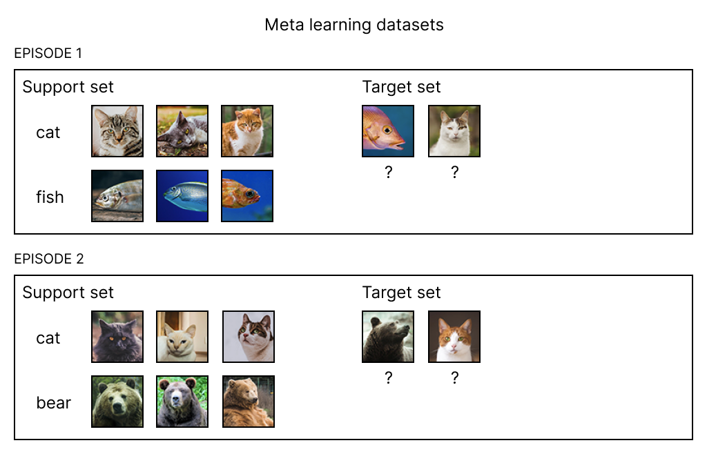
Papers in this field often use the notation of k and N, where k represents the number of opportunities the fast learner is given to learn, and N represents the number of classes it is required to be able to classify. Our running example, with N=2 and k=3, illustrates a two-way three-shot (N-way, k-shot) meta-learning setting.

Astute readers will notice that while our goal is to train a model to classify four classes (cat, bear, fish, and bird), each training episode only consist of two classes. This is a feature of meta-learning. The training procedure for meta-learning, first proposed by Oriol Vinyals in his seminal paper on matching networks is based on the principle that testing and training conditions must match. We do not show all classes to the fast learner at once because we expect the model to predict correctly (during inference) when shown a couple of images from a small number of classes. In addition, not all classes are used as training data. In our example, we might just use three classes, and expect the model to be able to make predictions accurately about the final class. Meta-learners can do that because they are trained to be able to generalize to other datasets. Each time the fast learner is shown an episode of data, it is exposed to a small subset of classes. The meta-learner cycles through many, many episodes, each exposing the fast learner to a different subset of classes. As a result, the fast learner not only learns to quickly classify each subset of classes, it also extracts the commonality and differences across all the classes.

Similarity between classes

If you were given a set of example images and were asked to classify a new image, the natural thing to do would be to compare the new image to the examples, find the one that is the most similar, and use its class as the new image’s label. This is the idea behind similarity-based approaches. To classify a new (target) image based on the examples available (the support set), first find its closest image from the examples, then use that image’s label as a prediction. In matching networks, images are represented by their embeddings, and distance between images is simply cosine distance between image embeddings. Embeddings, which we discussed in the context of languages in our “Summarization” and “Semantic Recommendations” reports, are rich numerical representations of text that a computer can understand. For images, embeddings can be thought of as a group of features (lines, edges) that richly represent images. The goal of the matching networks approach, then, is to converge to embeddings that will result in the following: target image being closest to the support set image with the correct label.

When an image in the target set belongs to a new unseen class, the matching network model treats it like any other image. It links the new image to the closest image in the support set, and uses that image’s label as a prediction. The matching network works with new and unseen classes!

Internal representation

In essence, the previous approach takes advantage of a distance metric based on embeddings to compare new images to example images in the support set. The model is trained such that we can correctly, in a probabilistic sense, link new images to one of the example images. Post-training, we end up with a model capable of generating representation of images (through embeddings) that captures both the difference and commonality between images. This suggests another approach to teaching machines to learn quickly with little training data. We start by finding a internal representation that can be adjusted easily with new tasks; the model can then rapidly adapt to new tasks using only a few datapoints.

In the context of deep learning, internal representation typically manifests itself as a set of parameters for the neural network. A “good” internal representation is one that is broadly suitable for many tasks. Small tweaks to this representation will produce a model that works well for new tasks. These tweaks are usually performed under the framework of transfer learning. Training the network using a small number of new datapoints while only adjusting weights at the final layers is an example of a feature extraction using transfer learning. Larger tweaks, where the entire model (or parameters) are re-trained using new datapoints is also possible, and is known as fine-tuning.

But where does this magical internal representation come from? In transfer learning, it is a pre-trained neural network from another task which has ample training data. Once initialized, the new, small dataset is used to re-train the network either fully or partially (just the final layers). An alternative way to arrive at this internal representation is through an initial set of network parameters. Once the network is initialized with the right parameters, it becomes quick and easy to adjust using a small number of new data. This implies that the initial set of network parameters should be sensitive to changes in the new tasks; small changes in the parameters will result in large improvements on the loss function of any task.

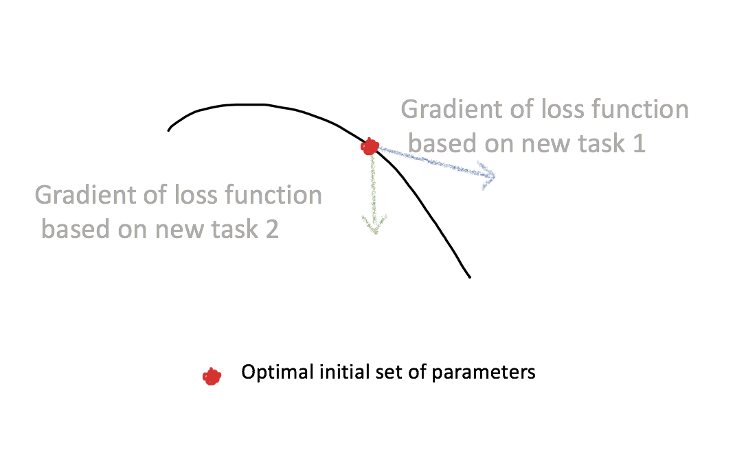
The general idea behind this approach is the following. We start with a model and its initial set of parameters. We train this model on a new task using data from an episode. During training, the initial set of parameters gets updated; it becomes an updated set of parameters. The goal is to find an initial set of parameters such that the loss, when measured on the new task, using the new set of parameters, is small.

This approach is inspired by transfer learning, but while transfer learning works for moderately sized datasets, it often becomes less effective in cases where datasets are too small or are too different from the original dataset used to create the pre-trained network. Optimization approaches in meta learning - optimizing for a set of initial parameters, or optimizing for the model to converge to a good solution rapidly on each task - attempt to come up with a systematic way to learn a common initialization that would serve as a good starting point for the possibly diverse tasks at hand.

The state of meta learning

Meta-learning is promising because it gets to the heart of the problem of learning with limited labeled data. Meta-learning, though, requires a different data collection paradigm. In traditional machine learning, we focus on collecting many examples of a class. In meta-learning, the focus changes to collecting many tasks. Indirectly, this implies the need to collect data for many diverse classes. In our example, we used four classes (cat, bear, fish, and bird) and defined a task to be “predicting one out of two classes when given three examples each”. This gives a maximum of six (four choose two) different tasks and is obviously insufficient for much learning to happen. Thus, in meta-learning, even though we do not need many examples of cats, we do need examples of many types of animals. Further, during inference, support and target sets typically need to be constructed as well. It is a different type of data requirement (or constraint) and can be expensive for certain use cases. Even within research, the datasets are limited to Omniglot and miniImagenet. The Omniglot dataset has a total of 1623 handwritten characters, each with 20 examples. The miniImageNet dataset consists of 100 classes from the original ImageNet dataset, each with 600 examples.

Meta-learning is an area that is quickly evolving, but it is not dominated by a single algorithm. The most promising class of algorithms seems to be based on optimization approaches; they are inspired by transfer learning and might see relatively quicker adoption. We expect meta-learning to become more important as the underlying algorithms become mature, particularly for use cases such as product classification or rare disease classification, where data exhibits many classes, but each class merely has a few examples.

Acknowledgement: We’d like to thank Oriol Vinyals for his insights.