Jun 22, 2020 · post

How to Explain HuggingFace BERT for Question Answering NLP Models with TF 2.0

Given a question and a passage, the task of Question Answering (QA) focuses on identifying the exact span within the passage that answers the question.

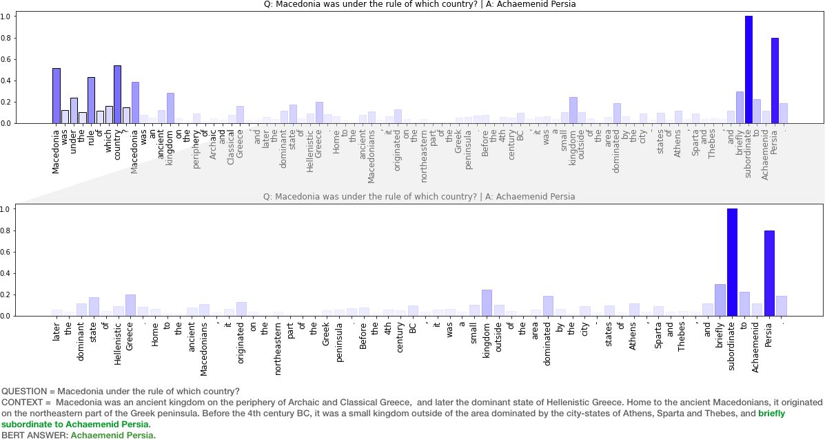
Figure 1: In this sample, a BERTbase model gets the answer correct (Achaemenid Persia). Model gradients show that the token “subordinate ..” is impactful in the selection of an answer to the question “Macedonia was under the rule of which country?". This makes sense .. good for BERTbase.

Recently, our team at Fast Forward Labs have been exploring state of the art models for Question Answering and have used the rather excellent HuggingFace transformers library. As we applied BERT for QA models (BERTQA) to datasets outside of wikipedia (e.g legal documents), we have observed a variety of results. Naturally, one of the things we have been exploring are methods to better understand why the model provides certain responses, and especially when it fails. This post focuses on the following questions:

• What are some approaches for explaining a BERT based model?
• Why are Gradients a good approach?
• How to implement Gradient explanations for BERT in Tensorflow 2.0?
• Some example results and visualizations!

Figure 2: In this sample, we use DistilBERT for the same question/context pair and get a different result! By looking at the gradients, we see that while the model sees the word subordinate as impactful, it also sees the word dominant as more impactful and selects an answer in that neighborhood. Bad for DistilBERT..

Code used for this post (graphs above) is available in this Colab notebook. Try it out!

How Do We Build An Explanation Interface for NLP Models like BERT?

From the human computer interaction perspective, a primary requirement for such an interface is glanceabilty - i.e. the interface should provide an artifact  - text, number(s), or visualization - that provides a complete picture of how each input contributes to the model prediction. There are several possible strategies for this. We can use model agnostic tools like LIME and SHAP or explore properties of the model such as self-attention weights or gradients in explaining behaviour.

Blackbox Model Explanation (LIME, SHAP)

Blackbox methods such as LIME and SHAP are based on input perturbation (i.e. remove words from the input and observe its impact on model prediction) and have a few limitations. Of relevance here is that LIME does not guarantee consistency (LIME local models may not be faithful to the global model) and SHAP has known computation complexity issues(KernelSHAP explores multiple combinations of input where a feature is present/absent …. computing these combinations can take a while). See this notebook for some additional discussion on these methods as well as their pros and cons.

We’ll skip this approach.

Attention Based Explanation

Given that BERT is an attention based model, it is tempting to use attention weights as a way to explain its behaviour. After all, attention weights are a reflection of what inputs are important to some output task [5]. This line of thought is not exactly bad, as attention weights have been useful in helping us understand and debug sequence to sequence (seq2seq) models [5].  However, BERT uses attention mechanisms differently (see this relevant article on self-attention mechanisms). While a traditional seq2seq model typically has a single attention mechanism [5] that reflects which input tokens are attended to, BERT (base) contains 12 layers, with 12 attention heads each (for a total of 144 attention mechanisms)!

Furthermore, given that BERT layers are interconnected, attention is not over words but over hidden embeddings, which themselves can be mixed representations of multiple embeddings. Recent research shows that each of these attention heads focus on different patterns (e.g. heads that attend to the direct objects of verbs, determiners of nouns, objects of prepositions, and coreferent mentions [1]). Each of these different attention patterns are combined in opaque ways to enable BERTs complex language modeling capabilities. This immediately brings up the challenge of deciding which (combination of) mechanism(s) to use for explaining the model. For additional details on visual patterns within BERT attention heads, see this excellent post by Jesse Vig.

Related research has also found that attention weights may be misleading as explanations in general [2] and that attention weights are not directly interpretable [3]. This is not to say attention weights are useless for debugging models .. far from it. They are valuable for scientific probing exercises [1] that help us understand model behaviour, but perhaps not as a tool for end user interpretability.

We will also skip the attention based explanation approach.

Gradient Based Explanation

It turns out that we can leverage the gradients in a trained deep neural network to efficiently infer the relationship between inputs and output. This works because, the gradient quantifies how much a change in each input dimension would change the predictions in a small neighborhood around the input. While this approach is simple, existing research suggest simple gradient explanations are stable, and faithful to the model/data generating process [4] compared to more sophisticated methods (e.g. GradCam and Integrated Gradients).

Let’s explore this approach!

Gradients in TF 2.0 via GradientTape!

Luckily, this process is fairly straightforward from a Tensorflow 2.0 (keras api) standpoint, using GradientTape. GradientTape allows us to record operations on a set of variables we want to perform automatic differentiation on. To explain the model’s output on a given input we can:

• (i) instantiate the GradientTape and watch our input variable
• (ii) compute forward pass through the model
• (iii) get gradients of output of interest (e.g. a specific class logits) with respect to the watched input.
• (iv) use the normalized gradients as explanations.

The code snippet above shows how these steps can be implemented  - where model is a Hugging Face BERT model and tokenizer is a Hugging Face tokenizer. Snippet is adapted from Andreas Madsen’s note on explaining a BERT language model using gradients. Full sample code can be found in this Colab notebook.

Visualizations below show some results from explaining 8 random question + context snippets.

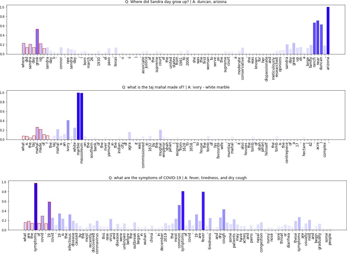
Figure 3: Additional examples of explanations via good old gradients!

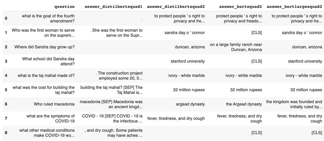
Figure 4: DistlBERT vs BERT base vs BERT large models for QA on eight random question/context pairs. (Answer span results may vary slightly across each run)

• DistilBERT SQUAD1 (261M): returns 5/8. 2 correct answers.
• DistilBERT SQUAD2 (265MB): returns 7/8 answers. 7 correct answers
• BERT base (433MB): returns 5/8 answers. 5 correct answers
• BERT large (1.34GB): returns 7/8 answers. 7 correct answers

Explanations like the gradient method above and model output provide a few insights on BERT based QA models.

• We see that in cases where BERT does not have an answer (e.g. it outputs a CLS token only), it generally does not have high normalized gradient scores for most of the input tokens. Perhaps explanation scores can be combined with model confidence scores (start/end span softmax) to build a more complete metric for confidence in the span prediction.
• There are some cases where the model appears to be responsive to the right tokens but still fails to return an answer. Having a larger model (e.g bert large) helps in some cases (see output above). Bert base correctly finds answers for 5/8 questions while BERT large finds answers for 7/8 questions. There is a cost though .. bert base model size is ~540MB vs bertlarge ~1.34GB and almost 3x the run time.
• On the randomly selected question/context pairs above, the smaller, faster DistilBERT (squad2) surprisingly performs better than BERTbase and at par with BERTlarge. Results also demonstrate why, we all should not be using QA models trained on SQUAD1 (hint: the answer spans provided are really poor).

In addition to these insights, explanations also enable sensemaking of model results by end users. In this case, sensemaking from the Human Computer Interaction perspective is focused on interface affordances that help the user build intuition on how, why and when these models work.

Conclusions: Whats Next? 

We have repurposed bar charts (not so good idea) to visualize the impact of input tokens on answer spans selected by a BERTQA. Perhaps an overlaid text approach (similar to textualheatmaps by Andreas Madsen) would be better. I am working on some user interface that ties this together and will explore results in a future post. There are also a few other potential gradient based methods that can be used to yield explanations (e.g. Integrated Gradients, GradCam, SmoothGrad, see [4] for a complete list). It may be interesting to compare explanations from each method.

References

• [1] Clark, Kevin, et al. “What does bert look at? an analysis of bert’s attention.” arXiv preprint arXiv:1906.04341 (2019).
• [2] Jain, Sarthak, and Byron C. Wallace. “Attention is not explanation.” arXiv preprint arXiv:1902.10186 (2019).
• [3] Brunner, Gino, et al. “On identifiability in transformers.” International Conference on Learning Representations. 2019.
• [4] Adebayo, Julius, et al. “Sanity checks for saliency maps.” Advances in Neural Information Processing Systems. 2018.
• [5] Bahdanau, Dzmitry, Kyunghyun Cho, and Yoshua Bengio. “Neural machine translation by jointly learning to align and translate.” arXiv preprint arXiv:1409.0473 (2014).