Jul 7, 2021 · post

Exploring Multi-Objective Hyperparameter Optimization

By Chris and Melanie.

The machine learning life cycle is more than data + model = API. We know there is a wealth of subtlety and finesse involved in data cleaning and feature engineering. In the same vein, there is more to model-building than feeding data in and reading off a prediction. ML model building requires thoughtfulness both in terms of which metric to optimize for a given problem, and how best to optimize your model for that metric!

Perhaps we’re making an error-detection system for some sensitive industrial process with an extremely high cost of failure, so we want to flag all potential errors, even if they’re relatively low-probability. Recall would be an appropriate metric to optimize. In contrast, a spam detector had better be sure something is spam before it is removed from a person’s inbox, and so should be high precision. Choosing these metrics carefully allows us to iterate on a machine learning system quickly, without deploying and waiting to analyze the real world impact between iterations. We can use these metrics to select the best performing algorithm before we deploy.¹

For very easy problems, we can sometimes find a very good algorithm “out of the box,” using the default settings, or small modifications to the defaults, of our preferred machine learning software. More often, we must tune the hyperparameters of our algorithm to allow it to most effectively learn our chosen task. For instance, in a tree-based model, the maximum tree depth (how many splits are allowed) plays a crucial role in controlling the bias-variance tradeoff to avoid overfitting. Machine learning algorithms can have many such hyperparameters, and manually setting them all would be laborious, and certainly not guaranteed to yield good results. Fortunately, given a definition of a “good result,” we can rely on computational methods to select hyperparameters for us. This process is known as hyperparameter optimization (HPO).

Our Session-based Recommender Systems research report described how we can apply word2vec to non-natural language problems, by treating a person’s history of product purchases as a series of “words,” and framing the recommendation problem as next-”word” prediction. A key insight when applying word2vec in such a fashion is that hyperparameters matter (see the conveniently-titled Word2vec applied to Recommendation: Hyperparameters Matter). Tuning the hyperparameters of word2vec to extract a representation for use in the downstream recommendation task resulted in a substantial improvement in recall on that task (to say, better recommendations)!

For those session-based recommendation experiments, it was tractable to use grid search (via Ray Tune) to comprehensively scan over hyperparameters. However, we were pushing the computational limits of the modest hardware we ran those experiments on, and had we another hyperparameter to scan, we may well have run out of compute. Throughout those experiments we came across a plethora of new techniques in the hyperparameter optimization space and decided we absolutely needed to dig deeper. Not only that, the space is so vast that it became a research cycle of its own!

So far, we’ve mentioned the “usual suspect” metrics of predictive accuracy, recall, and precision, but a production model must often satisfy physical requirements as well. Hyperparameter optimization becomes even more challenging when we have multiple metrics to optimize. For instance, in our industrial process example, our algorithm may be operating on video feeds or a high frequency image stream, and possibly run on embedded hardware. While we still wish to optimize recall, we may also need to find a model that fits within the memory constraints of our equipment, and predicts with as little latency as possible.

This post will examine this “multi-objective” hyperparameter optimization scenario in detail. Before we get to that, there are two other research directions worth mentioning.

Research frontiers in hyperparameter optimization

Being such a commonplace part of the machine learning process, HPO may not seem a likely candidate for cutting-edge research. However, HPO is, after all, optimization, which is itself a whole field, akin to machine learning. The commercial applications of optimization are widespread, and its commercial value is attested to by the viability of proprietary optimization software: as of this writing, Wikipedia’s list of Proprietary software for optimization contains 47 libraries, platforms and languages. Entire companies do only optimization. As such, research progresses apace!

Bayesian Optimization / smarter search

Grid search gives, by definition, pretty comprehensive coverage of a hyperparameter space at some resolution. Alas, it’s not always computationally possible to search over a granular grid, since the number of hyperparameter configurations grows combinatorially with the number of hyperparameters.

When we are compute constrained, the first step towards a smarter search is random search. Random search has the benefit of allowing the programmer to specify a compute budget of a fixed number of trials (with grid search, one can only do this by tuning the grid to a certain coarseness such that the combination results in the right number of trials). It’s also trivially resumable—since none of the subsequent trials depend on the earlier trials, we can add more searches as time and compute permit. This would be possible with grid search, by filling in gaps in the grid, but a little harder to program.

Another benefit of random search is that it samples more values of each hyperparameter than an equivalent grid search. A 3x3 grid search over two hyperparameters samples 3 values of each hyperparameter, but for the same 9 total evaluations, we could evaluate 9 values of each hyperparameter. Thanks to this, random search often finds better results than grid search, for the same compute budget (see Random Search for Hyper-Parameter Optimization. Both grid search and random search are embarrassingly parallel.

However, both grid search and random search are naïve. When we try a hyperparameter configuration and observe properties of the resulting model, we learn something! We can improve our search using that information. A sensible framework for doing so is Bayesian optimization.

Bayesian optimization assumes that there’s a functional mapping between the input hyperparameters and the output objectives. When we try a hyperparameter combination by training a model and measuring the objective, we learn something about the mapping, and can update our model of the function (hence “Bayesian”—we’re updating our prior beliefs). This means we can select the next trial point more intelligently. By acknowledging the uncertainty in the mapping, we can address the explore/exploit tradeoff: do we “exploit” and sample in the neighborhood of a configuration that is currently maximizing our objective, or do we “explore” to reduce the uncertainty in another area of the search space, potentially finding a better region?

The drawback of Bayesian optimization is that it is inherently sequential. In order to determine the next best HP combination to evaluate, we must await the results of the current trial. Each trial relies on all previous trials to make the best estimate for the next HP configurations to test. While parallel Bayesian approaches exist, in this regime, a single trial does not have access to all past trials because the other trials are being run in parallel! The algorithm thus has less information when estimating the next best HP combination and the resulting suggestion may be subpar, compared to the non-parallel approach. It’s likely that more trials will be needed in order to overcome the mildly sub-par HP estimates. However, with enough compute, parallel approaches can still be faster than non-parallel approaches, even with this impediment (an observation also made in Algorithms for Hyper-Parameter Optimization, which is essential reading for folks interested in this space). We’ll give a more thorough introduction to BO below.

While we focus on Bayesian optimization in this post, it is far from the only approach to smarter hyperparameter search. Other successful optimization families include multi-fidelity optimization and population-based optimization. We recommend taking a look at Section 4 in On Hyperparameter Optimization of Machine Learning Algorithms: Theory and Practice for a comprehensive overview of each of these HPO families, including more details on specific algorithms that we don’t cover here. (Actually, the whole paper is a great resource for practical HPO!)

Distributed Optimization / bigger search

The software space for hyperparameter optimization is flourishing. Machine learning toolkits often provide some facility for HPO built-in, or tightly integrated. See, for instance, scikit-learn’s grid and random search, Keras’ Keras-tuner, and H2O’s grid search. Other libraries have adopted similarly high level interfaces to smarter search routines (among the simplest is scikit-optimize, which provides BayesSearchCV, a drop in replacement to scikit-learn’s RandomSearchCV implementing Bayesian optimization).

Since much of hyperparameter search is parallelizable, it makes sense that there’s a growing ecosystem of libraries for distributing HPO. Distributed systems are hard, but frameworks are evolving to make them easier for specific use cases, like HPO². Two particular open source frameworks that we’ve been exploring recently:

• Ray Tune is based on the Ray framework for distributed processing. Tune can support optimization over any machine learning framework, and provides specific integrations for several common ML utility libraries (TensorBoard and MLflow, for example).

• Dask ML is built atop the Dask distributed processing framework, which itself implements a subset of the pandas and scikit-learn APIs to support distributed processing. Dask supports distribution of both data and computation, allowing hyperparameter search even when the data does not fit in the memory of a single node.

With the rise of MLOps and broader operationalization of machine learning models, the distributed machine learning ecosystem is likely to bloom further. Given the rise of AutoML in particular, distributed hyperparameter optimization is likely to become increasingly commonplace.

Multi-objective Optimization

In practice, we may often optimize a machine learning algorithm for a single objective, but we rarely truly care about just one thing. Would we want a 99.99% accurate classifier if it took a week to make each prediction? Possibly, but it represents a very particular scenario. This is a little hyperbolic, but the essential point is true: we must always make tradeoffs between characteristics of algorithmic performance. While traditional characteristics include predictive performance metrics, there are often physical or ethical constraints that an ML algorithm must meet. Netflix famously ran a competition to find the best recommendation algorithm, but Netflix Never Used Its $1 Million Algorithm Due To Engineering Costs. Just as we may trade off precision and recall by changing the classification threshold, we can navigate the larger tradeoff space (predictive, physical, ethical) of a complete ML pipeline by optimizing the hyperparameters of the system. “Engineering cost,” as in the Netflix example, would be extremely tricky to encode, but prediction latency, serialized model size, and technical measures of fairness, for instance, are all fair game.

A particularly novel application of multi-objective hyperparameter tuning is aiding algorithmic fairness. There are many technical measures of fairness that are often in tension (see On the (im)possibility of fairness for a reasoned view of their mutual incompatibility). Multi-objective multi-fidelity hyperparameter optimization with application to fairness highlights that multi-objective optimization allows one to explore the empirical tradeoffs between those measures quantitatively. We may wish to trade off other metrics to meet a fairness threshold. Promoting Fairness through Hyperparameter Optimization explores the tradeoff of one fairness measure (equal opportunity) with accuracy for a real fraud detection use case.

As we’ll see in the next section, multi-objective hyperparameter optimization combines elements of everything we’ve talked about so far: smarter, bigger search over more objectives! But before we demonstrate some use cases, we need to understand a bit more theory.

The Pareto Frontier

We can frame the multi-objective optimization problem as a search for optimal tradeoffs. Let’s imagine that we really care about exactly two objectives: predictive accuracy, and the speed at which we can make a prediction.

Unfortunately, these things are likely to be in tension. It may be possible to construct a very accurate classifier by using extremely large models, or stacking several ML algorithms, or by performing many complex feature transformations. All of these things increase the computation necessary to make a prediction, and thus slow us down.³

Imagine we randomly sampled hyperparameter configurations and measured the speed and accuracy of the resulting models. We would surely find some configurations that result in algorithms being both slower and less accurate than others. Speaking technically, if one point—call it $A$—is better than another point—$B$—in one dimension, and at least as good in all other dimensions, we say $A$ dominates $B$. We’d never want to deploy dominated models, since there are other models that are strictly better in both the optimization objectives.⁴

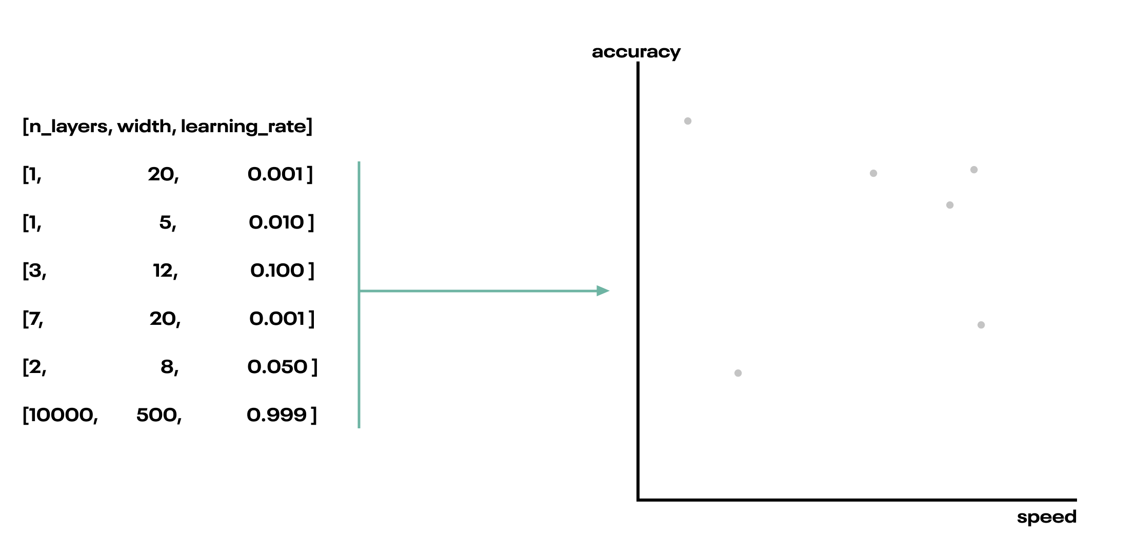Fig. As we try different hyperparameter configurations, we’ll find that the resultant models represent different accuracy-speed trade offs. We can visualize each model as a point in the trade off space.

It’s possible we’d find one point that maximizes both the accuracy and speed of our predictions. In practice, this is unlikely. We might improve accuracy by using deeper trees in a random forest, but deeper trees also take longer to evaluate, so we have traded off some speed for accuracy.

Eventually, we’ll discern an edge in the accuracy-speed tradeoff space, where we cannot find a hyperparameter combination that leads to an improvement in one direction without a negative impact on the other. This edge is called the Pareto frontier, and allows us to make a quantitative tradeoff between our optimization objectives. The Pareto frontier is constructed from the set of non-dominated points, and choosing any one of them gives us our exact accuracy/speed tradeoff.

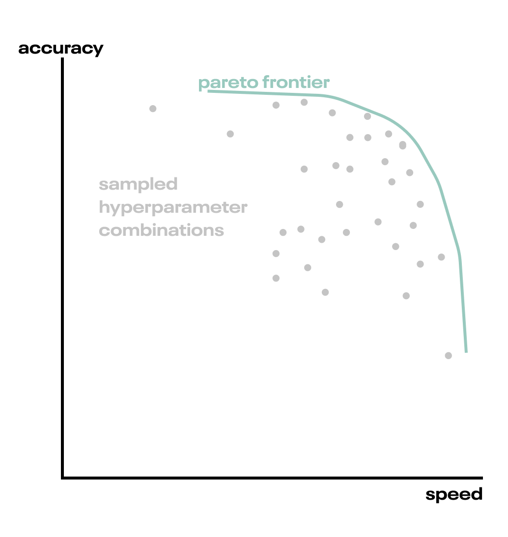Fig. The Pareto frontier is formed by those points that are not dominated by any others.

Ultimately, a deployed ML system will be trained with a single hyperparameter combination, and we must choose a single point in the accuracy-speed plane. The Pareto frontier allows us to present a decision maker with a host of models, some maximizing accuracy, others maximizing speed, and the entire spectrum in between.

How do we find this frontier? We could construct it as described above, with a dense random sampling of the hyperparameter search space. This risks being inefficient. We’d like to spend as little time as possible sampling configurations that aren’t likely to expand the Pareto frontier. Every sample on the frontier is useful, because they let us trade off accuracy and speed in a new combination. Samples inside the frontier end up being useless.

Multi-objective Bayesian optimization is a powerful technique (encompassing a collection of methods) for discovering the Pareto frontier. Rather than diving in at the deep end, let’s first review how Bayesian optimization works for a single objective. We’ll then build on that approach for the multi-objective case and discuss a few specific methods that we experimented with.

How Bayesian Optimization works

The “Bayes” in Bayesian optimization refers to updating our prior beliefs about how the input hyperparameters map to the output objectives, resulting in a better, posterior belief about the mapping. This approach to optimization is fundamentally sequential, and each iteration of the sequence follows the same procedure. The procedure looks like this:

• We have an unknown function between hyperparameters and our objective. We don’t know this true function (we’ll call it the objective function), but we can sample points from it by training a ML algorithm and evaluating the objective (calculating the accuracy, for instance). This is computationally expensive, so we’d like to do it as little as possible. Our goal is to optimize the output of this function, by which we mean to find it’s highest (or lowest, if appropriate) value.
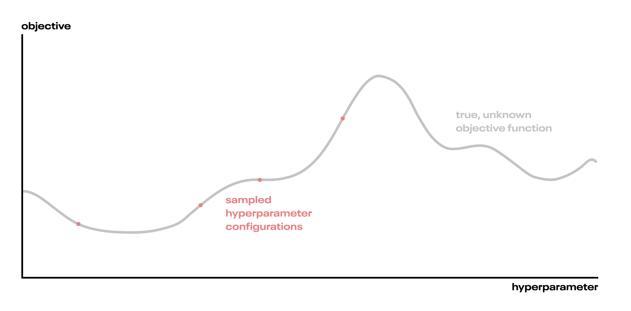
• Because we don’t know the true function, we fit a probabilistic surrogate function—usually a Gaussian Process (a class of flexible, non-parametric functions (technically, a stochastic process, which is a space of functions))—to some random samples from the objective function. It’s important that this surrogate function captures uncertainty.
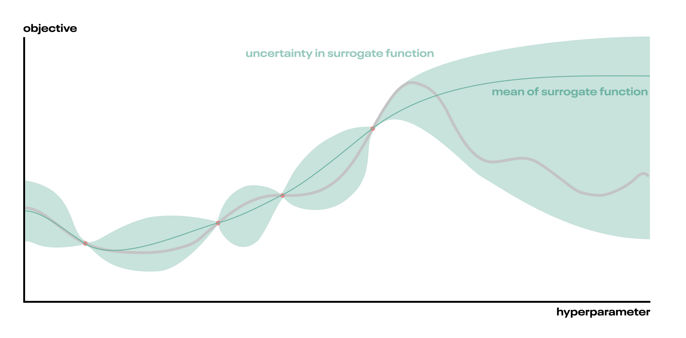
• From the surrogate function, we derive an acquisition function (if you’re counting, that’s the third function we’ve just introduced). The acquisition function tells us where in hyperparameter space to sample next. For instance, we might choose the point that has the highest probability of improving (PoI) the objective. Or, we might choose the point with the highest expected improvement (EI), which is different from PoI!
• Optimizing the acquisition function, for instance finding the highest EI, is itself an optimization problem! Fortunately, our surrogate function is very quick to evaluate compared to training a whole ML model, so we can find the highest EI point with iterative optimization methods. This inner loop of optimization is very fast.
• The optimal points of the acquisition function tell us where to sample next, so we evaluate our objective function at those hyperparameters and update our surrogate function with the output (making it a better model of the unknown, true objective function). Hence Bayesian optimization: we have a prior belief (the surrogate function) about the objective function, and we update that belief as we sample more points.
• We repeat this loop of updating the surrogate, calculating a new proposal point to sample, and evaluating the objective function. Eventually, we find an output of the objective function we’re happy with, or else blow our compute budget, and stop!

That’s a lot of functions. In a nutshell, we’re modeling the relationship between hyperparameters and objectives, and using that model to make better hyperparameter choices.

“Better” is doing some work there. When selecting a next datapoint to sample, we must make a tradeoff between maximizing the objective function as much as possible with the information that we have, and learning more about the objective function so we can make better future decisions. This is known as the explore-exploit tradeoff, and we navigate it by choosing an acquisition function. Each possible acquisition function determines the degree to which we explore and exploit the surrogate function. Some acquisition functions favour exploration of unsampled regions, others favour exploitation, and most have their own parameters to control the degree of exploration. A nice exploration of some acquisition functions is given in the Distill.pub article Exploring Bayesian Optimization (which is also a very accessible introduction to Bayesian optimization generally). If you’re unfamiliar with Gaussian Processes, we recommend first reading A Visual Exploration of Gaussian Processes.

We can overfit hyperparameters just as we can overfit parameters. When performing such a search, it’s a good idea to hold out an additional dataset for comparing models. This is true even with grid search. With grid or random search, we don’t explicitly “learn” a function, we just take a finite number of samples from it, but we might nonetheless pick a combination that is very good for the training set, and not so much for the test set. We can counter this by withholding an evaluation dataset split before starting any hyperparameter optimization, and using that dataset only for reporting our final metrics, not for choosing a model or finding the Pareto frontier.

That’s all the single-objective Bayesian optimization theory we need to understand the multi-objective case!

Further reading

This was a cursory summary of Bayesian optimization. A much more detailed, technical review is given in Taking the Human Out of the Loop: A Review of Bayesian Optimization. The excellent, standard textbook for Gaussian Processes is the freely available Gaussian Processes for Machine Learning (Rasmussen and Williams). This author has certainly not absorbed the whole book, but working through to chapter 2 should impart a sufficient understanding to use GP regression in a BO context. In case you are doubtful of the practical applications of Bayesian optimization, we point you to perhaps the most important work of scholarship on the subject, Bayesian Optimization for a Better Dessert.

Multi-objective Bayesian optimization

Since we now have a recipe for single-objective optimization, there’s an obvious solution to multi-objective optimization: we may reduce multi-objective optimization to a single objective case. We could do this by optimizing for a weighted combination of the two (or more) objectives, reducing them to a single number—a scalar—that we want to maximize or minimize. This is known as scalarization. Then, we can apply regular 1-dimensional optimization, and forget about there ever having been more than one objective.

This approach is only really viable if we have strong a priori quantitative knowledge about how much we care about each objective, since we must construct the precise combination to maximize. For instance, 2 * speed + accuracy, if we care about accuracy twice as much as speed. One reason this is hard is that the shape of the tradeoff is rarely known in advance. Are we prepared to sacrifice 10 points of accuracy for a 10 millisecond improvement in speed? How about 3 points of accuracy for a 100ms improvement? It is unlikely that we could confidently make these decisions without knowing what tradeoffs are available.

Maximizing a scalarized objective is going to hone in on a single point in the objective space (the speed-accuracy plane, for example). This is exactly one point on the Pareto frontier! So one way of discovering the Pareto frontier is by first optimizing for one point, then changing the weights in the scalarization, and repeating the procedure, each time optimizing for a different combination of accuracy and speed. Randomizing this combination is known, unsurprisingly, as random scalarization, and it forms the basis of the multi-objective optimization algorithm known as ParEGO.

It turns out it is possible to attack a multi-objective problem directly, without scalarizing, with a cleverly constructed acquisition function: the Expected Hypervolume Improvement.

Expected Hypervolume Improvement (EHVI)

The Pareto frontier generalizes the notion of optimizing to more than one dimension. But one can’t “maximize the frontier” – what does that even mean? To maximize (or minimize) a thing, we must have a notion of comparison between its possible values. For a single dimension, we compare magnitudes. How then, can we generalize comparison to multiple dimensions? By comparing volumes! Enter the Expected Hypervolume Improvement (EHVI) acquisition function. It’s perhaps best understood with a walkthrough.

Suppose we have a Pareto frontier of points initialized by randomly sampling the hyperparameter space. Even though these hyperparameter configurations were sampled randomly, we can still draw a Pareto frontier, which is just the set of points that are not dominated by others. We additionally choose a reference point that is completely dominated by the entire Pareto frontier (by every point on it). The hypervolume of interest is the volume occupied between the reference point and the Pareto frontier. With 2 objectives, the hypervolume is just the area. We are looking for points that increase this volume, which, intuitively, are points that push the Pareto frontier out, away from the reference point.

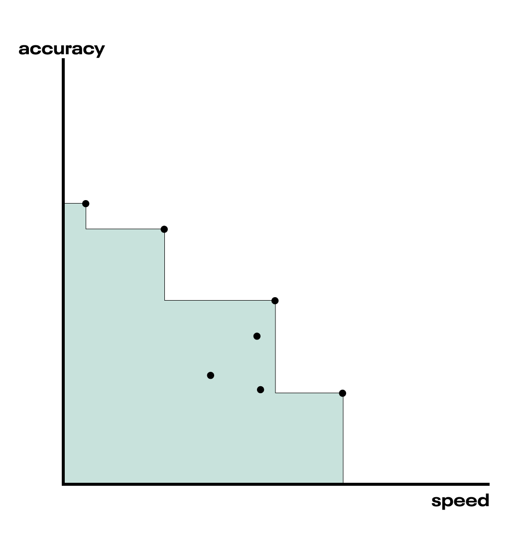Fig. The green shaded region is the hypervolume between the points on the Pareto frontier and the reference point, in this case, at the origin of the chart.

When we draw a new point, we sample from the hyperparameter space, but we want a volume improvement in the objective space. Our surrogate model – usually consisting of an independent Gaussian Process model for each objective – is approximating how input hyperparameters will result in output objective values, and the goal is to choose input hyperparameters that maximize the expected hypervolume improvement in the output space.

Choosing points that maximize the expected hypervolume improvement is itself an optimization problem, just like finding those that maximize expected improvement or probability of improvement in the single-objective case. We can perform this optimization using our surrogate functions, which are fast to compute. If we knew the objective function perfectly, the hypervolume improvement from adding a new point might look something like this.

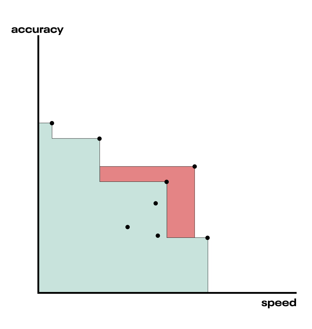Fig. The red shaded region is the hypervolume improvement that would result from adding the new candidate point.

However, we don’t know that objective function perfectly—we’re modelling it with surrogate functions (one for each objective). The surrogate functions come with uncertainty attached, since they’re just our best approximation of the objective function. Because of that uncertainty, we can’t be sure exactly where on the accuracy-speed space a given hyperparameter combination will land us, so the picture looks a little more like this.

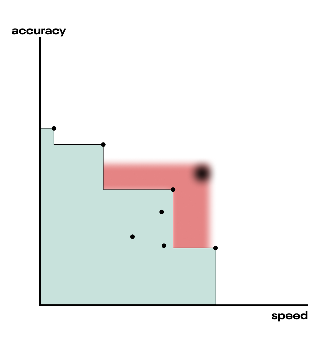Fig. In reality, we don’t know the objective function perfectly—we are modeling it with a surrogate function that has uncertainty. The fuzzy point and area on the chart indicate that the exact location of the point, and thus the associated hypervolume improvement, are uncertain.

This uncertainty is the reason we compute the Expected HVI, which means integrating over the uncertainty. There are fast computational methods for doing so using Monte Carlo and discretizing the space. Fortunately, evaluating the EHVI is not nearly as expensive as training an ML model and finding the true hypervolume improvement. So we can find the point that maximizes the EHVI using iterative methods (think BFGS). This is made all the faster by having exact gradients of the MC estimate of the EHVI, thanks to modern auto-differentiation tools.⁵

We evaluate the objective function at the suggested hyperparameters, and update our surrogate models. We can repeat this process for as long as our compute budget allows. By maximizing the hypervolume between the reference point (origin) and the Pareto frontier, we effectively construct the frontier itself!

Improvements to EHVI

There are two notable enhancements to expected hypervolume improvement. The first, qEHVI, allows for parallel suggested points. The second, MOTPE, replaces the GP models of the objectives with tree-structured Parzen estimators.

qEHVI

That little “q” signifies a recent advance – trying multiple new points in parallel – introduced in Differentiable Expected Hypervolume Improvement for Parallel Multi-Objective Bayesian Optimization, which also introduced the exact MC gradients mentioned earlier.

We need not restrict ourselves to trying only one new hyperparameter config at a time. The “q” in qEHVI indicates the number of parallel candidates suggested. The q candidates are selected by optimizing the total hypervolume improvement from their combined contribution, so they ought to work together. This makes sense, for if we chose three points that each maximize the EHVI independently, they’d be at the same spot. It’s a clever mechanism for exploiting parallelism in an otherwise sequential optimization process.

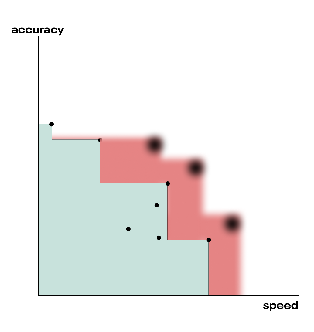Fig. qEHVI can suggest multiple (here q=3) new candidate points without refitting the surrogate models, accelerating the search for the Pareto Frontier.

The full technical treatment of qEHVI is given in the paper. We warn the intrepid reader that for anyone unfamiliar with Bayesian Optimization literature (which is vast and deep), and through no fault of the authors, the paper is a tough read. We recommend starting with this short video explaining the contributions of the paper.

Multi-Objective Tree-structured Parzen Estimators (MOTPE)

qEHVI improved on the EHVI acquisition function. An alternative approach is to improve upon the surrogate functions from which EHVI is calculated.

Gaussian processes offer a flexible approach to modeling which captures feature interactions. However, they are continuous in nature, and can struggle with awkward search spaces involving discrete transitions. An alternative approach known as Tree-structured Parzen Estimators (TPE) is superior for these spaces, and hyperparameter optimization often involves just such spaces. For example, the hyperparameter specifying the number of neurons in the third layer of a neural network is irrelevant if the hyperparameter specifying the number of layers is less than three in a given trial. GPs can model such functions with a continuous approximation, but the search space fundamentally is tree shaped.

Whereas GPs seek to model the probability of a given output (accuracy, for instance) conditional on the input hyperparameters $p(\text{accuracy} | \text{n_layers}, \text{learning_rate}, \dots)$, TPEs turn this around and model the conditional distribution of hyperparameters given the output:

$p\left(\text{hyperparameter} \ |\ \text{objective}\right) \ = \begin{cases} l & \mathrm{if} \ \text{objective} \ >\ \text{threshold}\\ g & \mathrm{if} \ \text{objective} \ < \ \text{threshold} \end{cases} $

The two functions $l$ and $g$ are themselves density estimations (“Parzen estimator” is just a particular name for a kernel density estimator), and functions of the hyperparameters. The threshold between them selects for whether the objective is among the best values, where “best” is defined as some upper quantile. A different density is fit to those good (upper quantile) objective values ($l$) and the poorer (lower quantiles) ones ($g$). New hyperparameters are drawn such that they’re very likely under the distribution $l$, and unlikely under the distribution $g$.

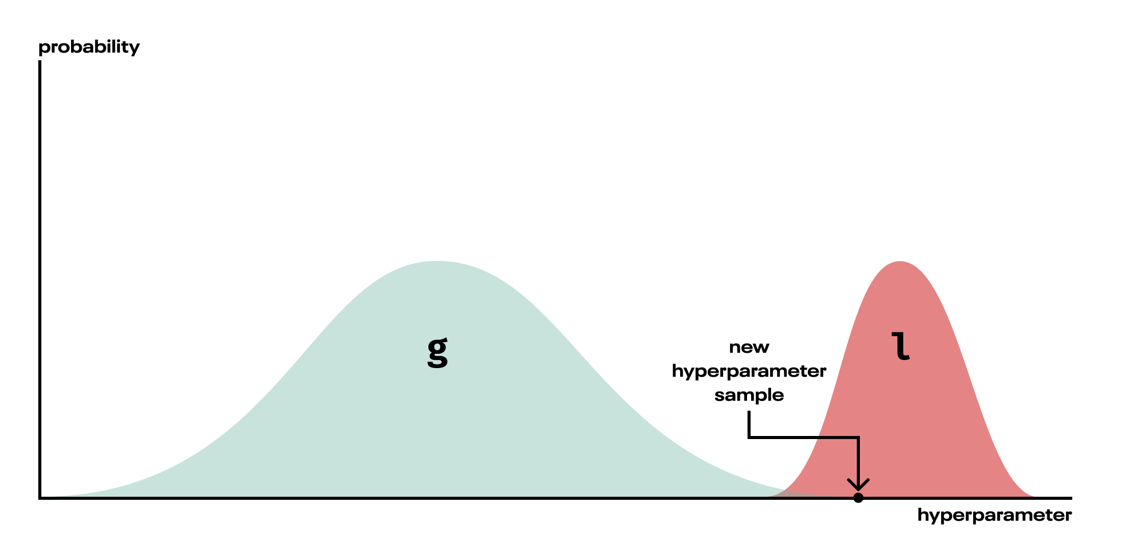Fig. TPE fits two densities to each hyperparameter, then samples hyperparameters from the configuration, l, that is fit only to the better objective values. In reality, the distributions may not separate so neatly.

Modeling the conditional distribution of each hyperparameter, rather than the objectives, means we can handle tree-shaped hyperparameter configurations such as the neural net example above. We simply don’t update the model, $p(\text{hyperparameter} | \text{objective})$, for a hyperparameter if it wasn’t used in a particular trial. As a trade off for this effective handling of tree-shaped search spaces, we lose the ability to model hyperparameter interactions, since each hyperparameter has its own conditional density. Whether this trade-off makes sense depends on the shape of our search space, and alas can rarely be known in advance.

Recently, Multiobjective tree-structured parzen estimator for computationally expensive optimization problems applied tree-structured Parzen estimators in the multi-objective case, using EHVI as the acquisition function. See Algorithms for hyper-parameter optimization for the introduction of TPE to hyperparameter search, and a comparison with Gaussian Process-based HPO.

Software

Mathematically speaking, Bayesian Optimization, and EHVI in particular, are not-trivial, to say the least. Fortunately, open source software for the purpose exists, and makes it considerably more approachable. We experimented with two software packages that facilitate multi-objective HPO: Optuna, and Ax.

Optuna

Optuna is a hyperparameter search package with a high level API that makes optimizing even relatively complex search spaces easy. This is enabled by its define-by-run nature that dynamically constructs a hyperparameter search space. Consider our earlier example of a neural network where both the number of layers and the width of each layer are hyperparameters. Optuna defaults to tree-structured Parzen estimators for modeling objectives (MOTPE in the multi-objective case), which handle this kind of space naturally. The high level of abstraction of the Optuna API is well-suited to practical hyperparameter optimization. When the model training process may already be complex, keeping the code surface of the optimization routine small is nice!

As a trade off to the flexibility of a define-by-run hyperparameter space, Optuna’s random search is suboptimal for problems with a fixed, non-dynamic hyperparameter space. It uses the numpy RandomState class to generate independent samples from the parameter space. As we’ll describe in our experiments, when the search space is not dynamic, there are substantially better-performing quasi-random sampling methods. In particular Sobol sampling seeks to cover the search space relatively uniformly (but not a strict grid). However, this operates by minimizing discrepancy (a measure of how non-uniformly distributed samples are) in a unit hypercube, which must be defined up front. There is ongoing work to integrate Sobol sampling for static search spaces, optuna/issues/1797, and in general the library is actively maintained and developed.

Optuna is our recommended library for almost all multi-objective hyperparameter optimization problems.

Ax

Before discovering Optuna’s multi-objective capabilities, we spent a lot of time with Ax. Ax self-describes as an “adaptive experimentation platform” for industrial grade optimization and experimentation. It provides several levels of abstraction appropriate for a variety of optimization tasks, including (but very much not restricted to) hyperparameter optimization.

The optimization algorithms (like qEHVI) for Ax are implemented in the lower-level BoTorch framework. BoTorch provides primitives useful for building novel Bayesian Optimization routines, taking advantage of the fast tensor computation and automatic differentiation provided by PyTorch. BoTorch is primarily useful to optimization researchers, and we restricted our use to the higher level Ax platform.

Ax is extremely flexible, being a platform for generic black-box optimization. However, that flexibility incurs some overhead for our specific use case, multi-objective hyperparameter optimization. Multi-objective optimization is currently only supported by the low-level Developer API, the use of which involves understanding the granular abstractions used under the hood of the higher-level APIs. Multi-objective optimization is on the roadmap for the higher-level Service API though, which is likely to radically simplify Ax’s use for this case, and may additionally facilitate parallelization of multi-objective optimization with Ray.

One area that Ax shines is the inclusion of quasi-random Sobol sampling. In our experiments, we found this to be an extremely strong baseline, to the point that the additional complexity of qEHVI was rarely worth it when running fewer than 100 trials. We’d recommend Ax for those with complex optimization needs (such as human-in-the-loop), and with the caveat that, being a black box optimization framework applicable to almost any optimization problem, it is not particularly honed for hyperparameter optimization.

Like Optuna, Ax has active and responsive maintainers, and we’re excited about future developments for the library and ecosystem.

Experiments

To truly understand the multi-objective hyperparameter optimization (MO HPO) problem, we needed to experiment. We chose three problems on which to apply MO HPO, and provide notebooks tackling them below. The three problems were:

• A synthetic classification problem. These notebooks provide a tutorial on applying Optuna and Ax to MO HPO.
• A Credit Card Fraud dataset, sourced from Kaggle.com. This is a highly imbalanced problem, and fraud detection for in-flight transactions is a realistic scenario in which one cares both about predictive performance and prediction latency.
• Approximate Nearest Neighbor search. For large vector spaces, ANN search algorithms embody clear tradeoffs between recall, query time and memory consumption, for which we anticipated being able to find a well-defined Pareto frontier.

Synthetic data

To get to grips with Ax and see multi-output Bayesian optimization in action, we tackled a totally synthetic problem, generated by sklearn. Check out our notebook walkthrough below:

Ax on synthetic data

While we wanted to demonstrate how to use the Ax Developer API to do this, we’d actually recommend using Optuna for this kind of problem. This trades off the flexibility of Ax for a much smaller and simpler API. Check out the same demo with Optuna here:

Optuna on synthetic data

Credit card fraud

The synthetic data notebooks demonstrate how to use the libraries on a completely toy problem. What happens when we up the problem complexity a little and try a real machine learning problem? Here, we attacked credit card fraud detection using a dataset released by the machine learning group at Université Libre de Bruxelles. Credit card fraud comes with some interesting facets, such as a highly imbalanced class distribution. The same group recently released a handbook about the problem, for those interested in diving deep.

Credit card fraud

We put quite some effort into prototyping with xgboost and multi-layer perceptron algorithms on this dataset, with both Ax and Optuna. While we could cherry-pick results that show EHVI outperforming random search in finding hyperparameter combinations resulting in good, high AUPRC, low-latency algorithms, we couldn’t reliably reproduce these results, and often random would win.

Our working hypothesis is that the problem is essentially too easy, by which we mean xgboost could find a good solution under a wide range of hyperparameters. If only one or two hyperparameters are important to a problem, we can get good coverage of those with random sampling, or even a parameter sweep (tantamount to grid search). While Bayesian optimization might sample slightly more densely from the good region, it doesn’t provide a reliable substantial improvement (and indeed, it appears to trade off some exploration for that). We expect Bayesian optimization to shine when more than one hyperparameter is important and good coverage of the hyperparameter space is not possible.

Approximate Nearest Neighbors

Our final notebook dives deep into the world of approximate nearest neighbor (ANN) search. Approximate nearest neighbor search has all the elements we’re looking for: a real-world use case, a substantial and non-trivial dataset, and algorithms that have inherent tradeoffs between competing objectives like recall, inference time, and memory consumption. In this notebook we apply Optuna HPO to three different ANN algorithms on over one million GloVe word embeddings.

Approximate nearest neighbors

Again, we put a ton of effort into prototyping with these algorithms but the results weren’t impressive. In nearly all cases, random search performed about as well as Optuna’s MO HPO strategy. We surmise that the reason lies in the relationship of these algorithms’ hyperparameters with the output objective space. Many ANN algorithms have hyperparameters that are designed to exert influence on only one or two objectives, constraining the range of possible output realizations. For example, we may think we have a wide two-dimensional plane of (speed, accuracy) points to explore, like we’ve discussed above. But for ANNs, the reality is that the actual possible range of realizable values is quite narrow because ANN hyperparameters tightly control single objectives. When this happens, it becomes much easier for random search to perform about as well as a more sophisticated HPO strategy, because there’s simply less output objective space to explore.

Conclusion

Let’s recap. We introduced Bayesian optimization, especially as it applies to finding good hyperparameters for machine learning algorithms. We generalized to optimizing multiple objectives by choosing a clever acquisition function, the expected hypervolume improvement. We briefly discussed some software that enables multi-objective hyperparameter optimization, and then performed a host of experiments. What did we learn?

The traditional wisdom is that Bayesian Optimization should beat random search initially, when only a low number of trials are run (which is desirable, since trials are expensive), whereas random search will eventually explore the whole hyperparameter space, and win in the high-sample regime, though this may require many thousands of samples. This is also the empirical conclusion of Bayesian Optimization is Superior to Random Search for Machine Learning Hyperparameter Tuning: Analysis of the Black-Box Optimization Challenge 2020, which details a thorough study of Bayesian optimization applied to single targets on some scikit-learn datasets.

Our work here was exploratory, and we certainly can’t draw a robust conclusion without a benchmark suite and standard errors, but we were surprised to find that Bayesian optimization for multi-objective HPO did not consistently beat random search for the problems we attempted. There are numerous reasons this could be, and we give some discussion above and in the experiment notebooks themselves. Perhaps the problems were too simple, or only a couple of hyperparameters mattered, or, since this was far from a rigorous benchmarking, perhaps we merely witnessed some lucky random draws. One thing we learned is that, so long as your hyperparameter space is fixed, quasi-random Sobol sampling (as implemented in Ax) is an extremely strong baseline. Sobol sampling features the high coverage of the hyperparameter space, like grid search, but with the same benefit as random search of not repeating hyperparameter values.

The multi-objective Bayesian optimization methods we tried certainly worked in the sense of sampling the hyperparameter space more densely around the Pareto frontier (at least, by visual inspection of the resulting charts). However, the random nature of random search often eclipsed this benefit by sampling more widely. After all, there’s little benefit to samples that result in models that are too similar in their performance characteristics.

Recently, An Empirical Study of Assumptions in Bayesian Optimisation shed some light on the difficulty of hyperparameter optimization, especially for techniques that use Gaussian Processes for the surrogate function, like the Ax implementation of EHVI. GPs have a lot of baked-in assumptions (principally: stationarity and homoscedasticity, both of which can be handled by GPs, but are often not handled in BO frameworks) that don’t always hold true in real-world ML model hyperparameter optimization problems, further complicating an already challenging task.

Optuna’s EHVI implementation uses tree-based parzen estimators for the surrogate function which doesn’t come with the same set of assumptions. But, as we found in our approximate nearest neighbor experiments, the problem is still tricky, indicating that choice of surrogate function isn’t the only thing contributing to the ultimate success of HPO. The shape of the data, choice of algorithm, and the relationship between that algorithm’s hyperparameters and the output objective space all play a part in the success of multi-objective Bayesian optimization on a given use case. And, unfortunately, it’s unclear how to know before-hand whether your particular setup embodies qualities that will allow multi-objective Bayesian optimization to perform optimally.

Therefore, based on the experiments we’ve tried and the research we’ve reviewed, our recommendation is to start with a random search for MO HPO. If the HPO software suite you’re using includes a Sobol random sampling option, start with that. Move on to more sophisticated algorithms if you have a large compute budget or if small gains in the Pareto frontier of your tradeoff space translate to large gains in a physical application (e.g. 1% speedup on model inference translates to a 1% reduction in website churn).

We hope this exploration of multi-objective HPO left you with some useful knowledge to exploit! 😉⁶

If you’d like to hear more from us, follow us on Twitter, and sign up to our newsletter.