Jun 9, 2021 ·
Deep Metric Learning for Signature Verification
In our previous blog post, we discussed how pretrained models can serve as strong baselines for the task of signature verification. Essentially, using representations learned by models trained on the ImageNet task allowed us to obtain competitive performance when attempting to correctly classify signature pairs as genuine or forgeries (with ResNet50: 69.3% accuracy on skilled forgeries, 86.7% on unskilled forgeries).
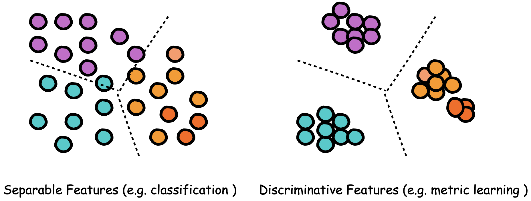
Figure 1. Metric learning allows us to learn a discriminative embedding space that both maximizes inter-class distance and minimizes intra-class distance.
However, several intuitions suggest that we might be able to improve on this. First, given that the pretrained model was trained on data (natural images), which does differ from our task data(signature images), it makes sense that some sort of fine-tuning would be useful in adapting the pretrained model weights to our data distribution. Second, the pretrained model is based on a classification objective (cross-entropy loss) - i.e., correctly classify one million images into 1000 different classes. It learns to maximize inter-class distances such that features before the softmax fully connected layer are linearly separable.
While this objective yields semantic representations that have proven to be useful, our primary task of verification does require something more precise. Essentially, we want an objective focused on capturing the similarities/dissimilarities between two data points; we want to learn discriminative features that not only maximize inter-class distance but also minimize intra-class distance. To achieve this goal, we can turn to metric learning: learning a distance metric designed to satisfy the objective of making representations for similar objects close and representations for dissimilar objects far apart, in some metric space.
What is Metric Learning?
A simple description of metric learning is “any machine learning model structured to learn a distance measure over samples”. The intuition here is that if the model is designed to learn a distance function for similar/dissimilar objects, we can use it for applications such as signature verification that rely on this property.
The metric learning objective can be formulated in several ways, depending on how the training dataset is structured.
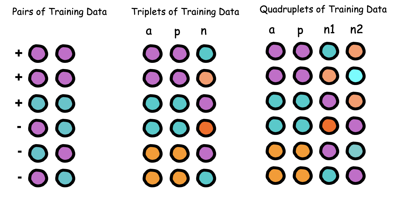
Figure 1.1. Data used to train a metric learning model may be structured as pairs, triplets, or quadruplets. This, in turn, influences how the loss function is designed.
Commonly, sets of training examples are structured as either pairs, triplets, or quadruplets, from which a distance function is learned. Despite the differences in problem formulation, the high-level metric learning workflow remains consistent:
- Define a dataset of train samples (2, 3, 4 data points in each sample, depending on loss function).
- Extract representations for each datapoint in a given sample, using a trainable embedding model. (Note that the exact architecture of this embedding model might vary depending on the data - e.g., a CNN architecture might be used for metric learning on images, while an RNN architecture might be useful for sequences.)
- Measure the similarity between data points in each sample using a distance function (e.g., Euclidean).
- Calculate a loss based on the observed vs. expected distances between data points. (For example, for data points we know to be similar - i.e., expected small distance - we have very little or no loss if their observed distance is indeed small.)
- Backpropagate the loss through the embedding network, so the model learns to produce similar representations for similar examples and distant representations for dissimilar examples.
In the following sections, we will consider a few loss functions for implementing metric learning.
Contrastive Loss
Contrastive loss (also known as pairwise ranking loss) is a metric learning objective function where we learn from training data examples structured as pairs: positive pairs (examples that belong to the same class) and negative pairs (examples that belong to different classes).
Note that the forged signature may be unskilled (i.e., the forger knows nothing about the original) or skilled (i.e., the forger has access to what the original signature looks like and actively attempts to mimic it). Clearly, it is easier to detect unskilled forgeries compared to skilled forgeries, which are hard to detect (even for humans). As we construct training pairs for a model to learn from, we want it to be particularly good at solving the hard version of the problem: distinguishing skilled forgeries.
In the contrastive loss setting, negative pairs consisting of unskilled forgeries are termed easy negatives, while those consisting of skilled forgeries are termed hard negatives.
The contrastive loss function is set up such that we minimize the distance between embeddings for positive pairs, and maximize the distance between embeddings for negative pairs. After each pass through the network, we ideally want to update the weights of our embedding model such that the above condition is satisfied. Contrastive loss can be implemented using a Siamese network architecture for the embedding model. This model takes in two inputs and uses a shared trunk network that produces two embeddings for each input.
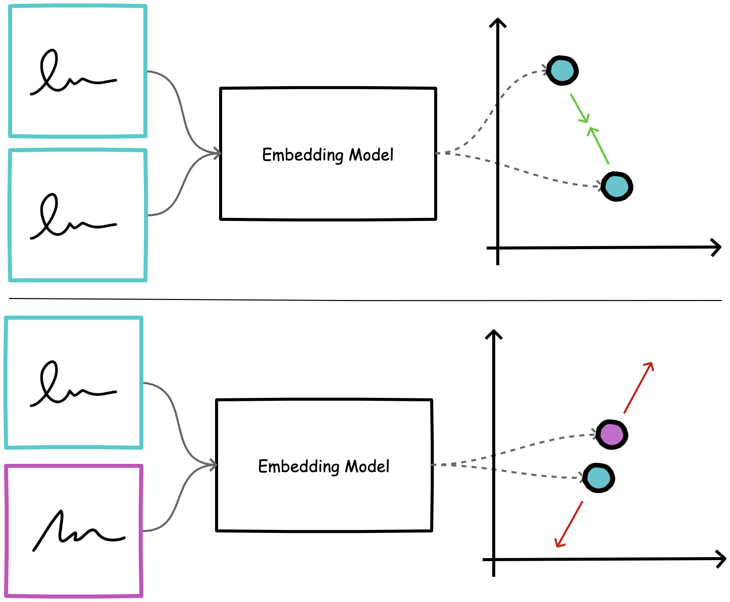
Figure 2. Contrastive loss is used to minimize the distance between genuine signature pairs (top) and maximize distance between negative pairs (bottom)
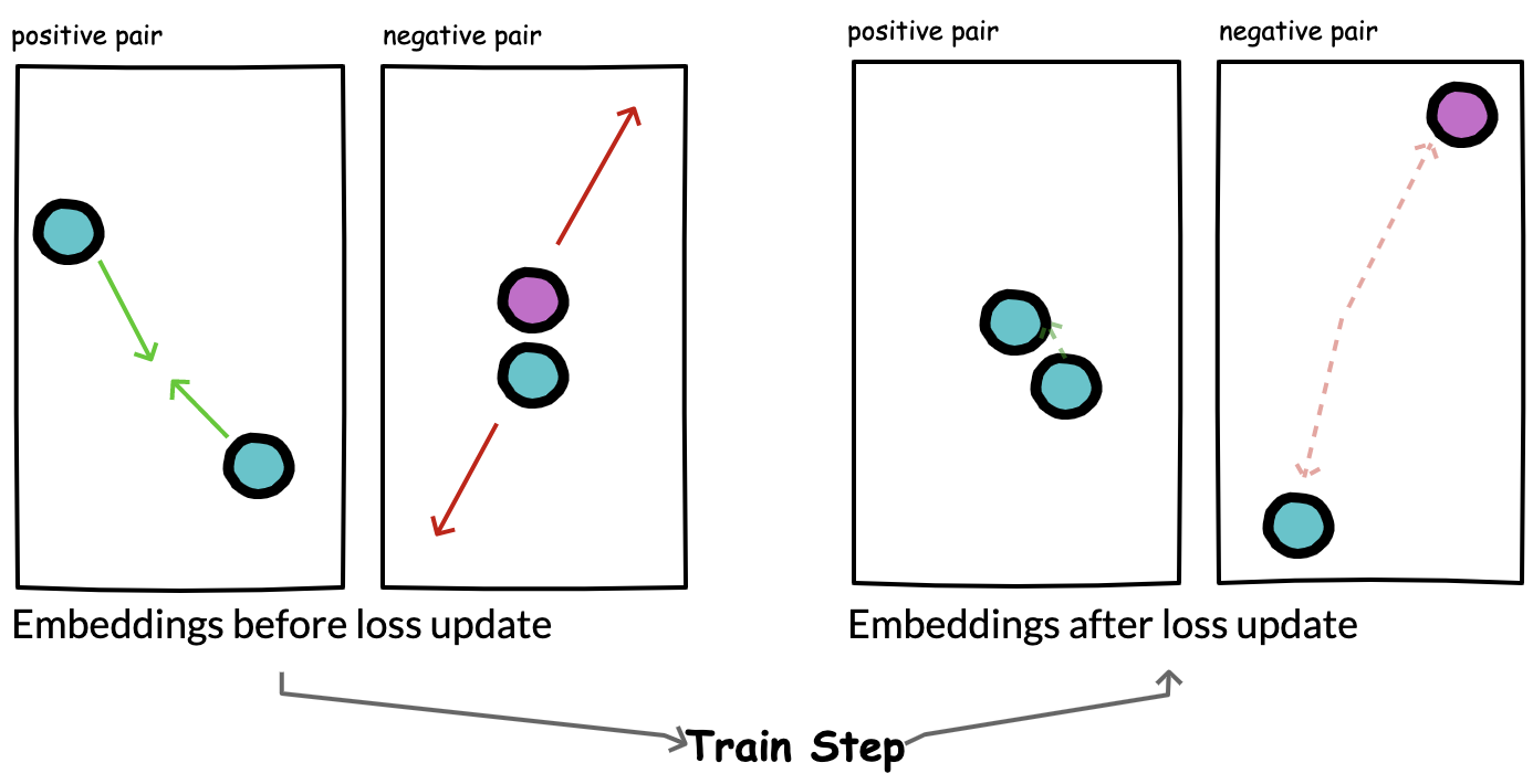
Figure 3. During training, we expect that loss updates will cause the model to update its weights such that positive pairs are closer and negative pairs are farther apart.
Contrastive loss is defined as:
$ Loss = \begin{cases} D \text{ ............................... if pair is positive}\\ max(0, m-D) \text{ ......... if pair is negative }\\ \end{cases} $
where $D$ is the calculated distance between embeddings for each datapoint in the pair, and $m$ is a constant value of margin.
In the case of positive pairs, the loss becomes positive only when we have a positive distance between vector representations. In the case of negative pairs, the loss is positive only when the distance between vectors is less than the margin. The margin value is a hyperparameter that serves as an upper threshold to constrain the amount of loss attributed to “easy to classify” pairs. A simple way to think about the function of the margin is that if the network produces representations that are distant “enough” for a given pair, there is no need to continue focusing training efforts on that example. 1
While contrastive loss is useful, it has a limitation. For points in a negative pair, contrastive loss will push them far apart without any knowledge of the broader embedding space. For example: imagine we have 10 classes, and each time we see class 1 and 2, we want to push them far apart; a result of this is that 1 might now become farther from 2 on the average, but might overlap with other classes (such as class 3, 4, 5, etc.).
Triplet loss addresses this issue by using triplets in each training sample: an anchor, a positive (same class), and a negative (different class) data point. This way, with each gradient update, we learn to minimize anchor + positive distance while also ensuring that the anchor is far from the negative point.
Triplet Loss
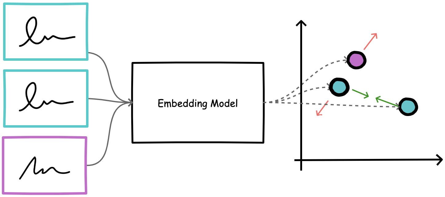
Figure 4. A triplet model is trained with triplets such that the distance between the anchor and positive is minimized while the distance between the anchor and negative is maximized.
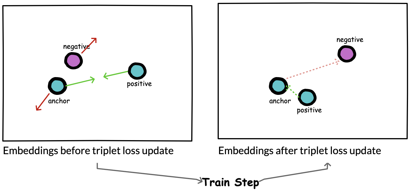
Figure 5. At each train step, we expect that triplet loss updates will simultaneously minimize the distance between anchor and positive while maximizing distance between anchor and negative samples.
The triplet loss function aims to learn a distance between representations such that the anchor-to-positive distance is less than the anchor-to-negative distance. Similar to contrastive loss, a margin value is imposed on the anchor-to-negative distance so that once negative representations have enough distance between them, no further effort is taken to increase distance between them. With this understanding, triplet loss is formally defined as:
$ Loss = max (0, m + D_p - D_n) $
where $D_p$ is the anchor-to-positive distance and $D_n$ is the anchor-to-negative distance and $m$ is the margin. With this loss formulation, we can create three different types of triplet combinations based on how we sample:
- Easy triplets: result when
$D_n$>$D_p$+$m$. Here, the sampled anchor-to-negative distance is already large enough so loss is 0, and the network has nothing to learn from. - Hard triplets: result when
$D_n$<$D_p$. In this case, the anchor-to-negative distance is less than the anchor-to-positive distance, meaning high loss to backpropagation through the network. - Semi-hard triplets: result when
$D_p$<$D_n$<$D_p$+$m$. Semi-hard triplets occur when the negative example is more distant to the anchor than the positive example, but the distance is not greater than the margin. This, therefore, results in a positive loss (i.e., the negative is far … but not far enough.) 1
Based on the above, we can see that different approaches for selecting triplets (also called triplet mining approaches) are not equally informative. More importantly, if we prescriptively mine the right types of triplets that are informative, we can increase the overall efficiency of learning. Ideally, we want to focus on hard and semi-hard triplets - a luxury we were not afforded in the contrastive, pairwise learning setup.
From Offline to Online Triplet Mining
To implement any of the triplet strategies, we need to obtain embeddings for our samples, so as to determine their distances and how best to construct our triplet. An initial offline approach will be to obtain embeddings for our entire training set, and then select only hard or semi-hard triplets.
Assuming we have a training set of size $T$:
- Get all embeddings for all points in
$T$ - Get a list of all possible
$T^3$triplets in$T$, and identify valid triplets (hard or semi-hard), based on embeddings and class labels - Compute loss and update model weights using valid triplets
This approach is inefficient, as it requires that we extract embeddings for the entire training set to generate valid triplets. It also assumes we have an embedding model that yields good embeddings on the train dataset prior to training.
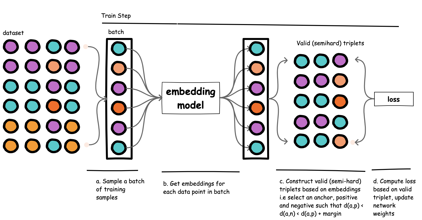
Figure 6. In online triplet mining, triplets are constructed during training.
We can be more efficient about this by adopting online triplet mining. 2 Here, we select our triplets during training (within each training batch), as opposed to precomputing triplets prior to training.
Assuming we have a batch of size $B$:
- Get embeddings for all
$B$data points in our batch - Get all possible triplets
$B^3$in$B$and identify valid triplets (hard or semi hard) based on embeddings and class labels - Compute loss and update model weights using valid triplets
As we will see later on, the ability to sample intelligently and introduce relative knowledge between three examples helps improve training efficiency, and results in more contextually robust feature embeddings.
Other Losses: Quadruplet Loss, Group Loss
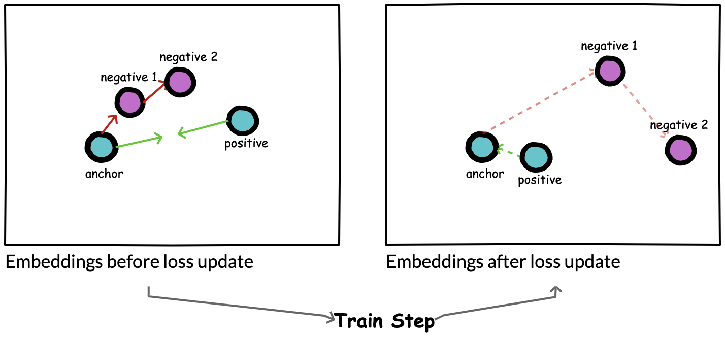
Figure 7: Quadruplet loss
At this point, it is clear that a good loss function should attempt to learn similarity using information from each training sample. Contrastive loss learns from pairs of images (positive, negative). Triplet loss achieves even better performance by simultaneously learning from carefully selected image triplets (anchor, positive, negative) within a batch. But what if we could simultaneously learn from even more samples within a batch? Existing research has explored this.
In their work, Chen et al. 2 3 introduce quadruplet loss, where each training sample consists of 4 data points (anchor, positive, negative1, negative2), where negative2 is dissimilar to all other data points. They minimize the distance between anchor and positive, while simultaneously maximizing distance between anchor and negative1 as well as negative1 and negative2.
Elezi et al 4 take this one step further and propose group loss, which aims to simultaneously learn from all samples within a minibatch (as opposed to a pair, triplet or quadruplet). To create the mini-batch, they sample from a fixed number of classes, with samples coming from a class forming a group. Thus, each mini-batch consists of several randomly chosen groups, and each group has a fixed number of samples. An iterative, fully-differentiable label propagation algorithm is then used to build feature embeddings, which are similar for samples belonging to the same group, and dissimilar otherwise. The overall effect of this group loss formulation is to enforce embedding similarity across all samples of a group, while simultaneously promoting low-density regions amongst data points belonging to different groups.
One trend we can observe from these loss functions is that the more data points from multiple classes we use to update our gradients, the better our model is able to capture the global structure of the embedding space. In theory, quadruplet loss and group loss represent the state of the art in metric learning loss functions, but they do introduce multiple parameters that can be challenging to implement and tune. Even when this is done correctly, the expected increase in performance (~1 - 4%) may be hard to reproduce, especially due to the stochastic nature of DNN training. In practice (as we will see in the experiment section below), triplet loss (with online learning) is efficient and high-performing; hence, it is the recommended approach.
Our Experimentation
Dataset
To evaluate a metric learning approach on our signature verification task, we experimented with contrastive and triplet loss. We first constructed an experimental setup consistent with the design from our pretrained baseline experiment. Using the CEDAR dataset, we withheld signatures for 11 of the 55 authors as a test set, and used the other 44 as a training set.
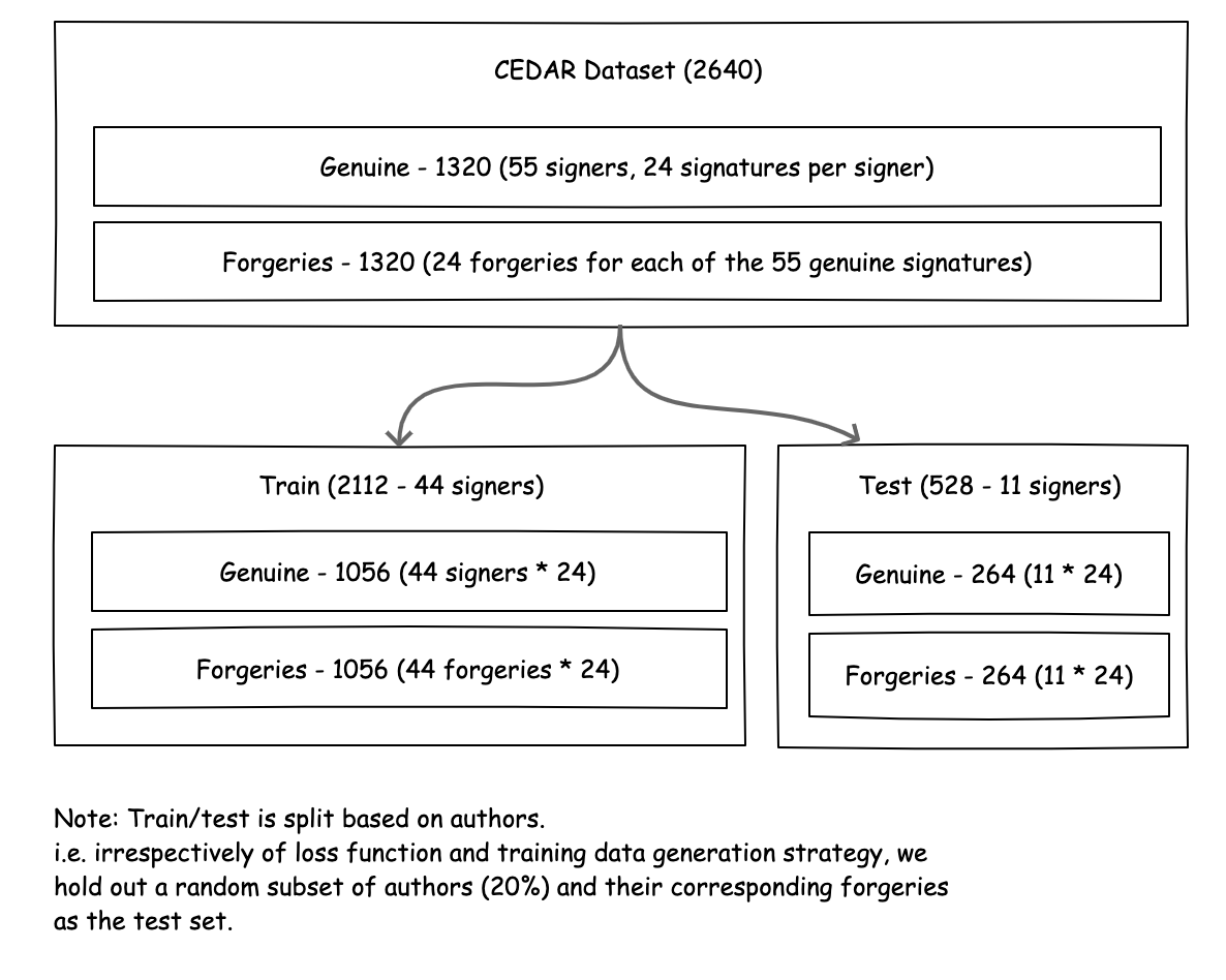
Figure 8. The CEDAR dataset used for our signature verification experiments.
Note that depending on the loss function, the strategy for constructing the eventual training dataset from which the network learns might differ. In our contrastive loss experiments, we generated a total of 36,432 pairs. For our triplet loss experiments - given that we used the online triplet mining approach - we structured the dataset as a classification problem; each signer and each forgery was treated as a class, making for a total of 88 classes with 24 samples (2112 total), each in the training set. Amongst other limitations, the CEDAR dataset is small; as we’ll see later on, this makes it challenging to train a performant neural network from scratch.
To evaluate each model, we constructed a set of pairs of positives and negatives (see Figures 9 and 10 for examples of skilled and unskilled forgeries in our test set) and report maximum accuracy and equal error rate. Except where mentioned, the performance scores we report are based on a test set of positives and skilled forgeries (hard negatives). (Additional discussion on evaluation metrics is provided in a previous post in this series.)
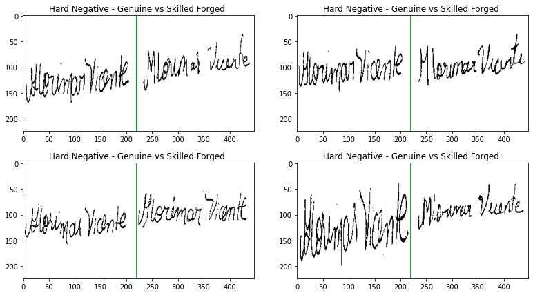
Figure 9. Examples of skilled forgeries where the forger has access to the genuine signature and attempts to replicate it. We refer to such pairs as hard negatives. All performance scores reported are based on a test set containing this type of negatives.
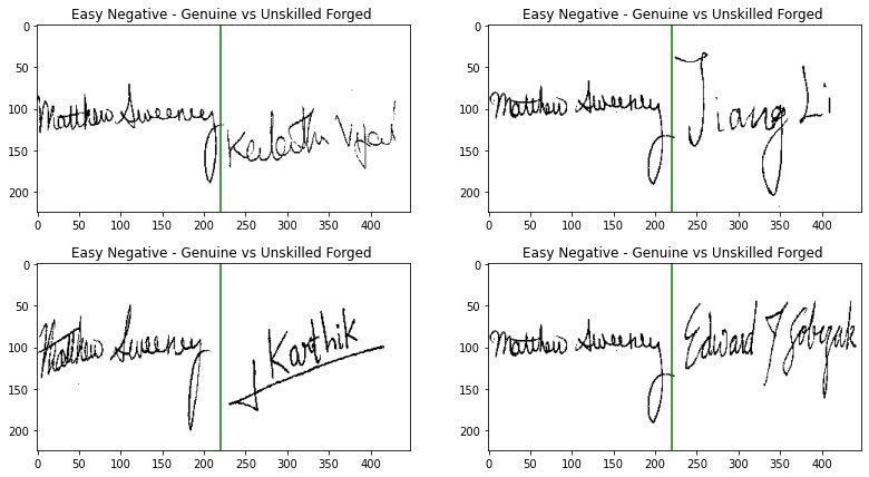
Figure 10. Examples of unskilled forgeries where the forger does not have access to the genuine signature and may provide a random signature instead. We refer to such pairs as easy negatives.
Contrastive Loss Training and Evaluation
For contrastive loss, a Siamese network was assembled, using an embedding model composed of a frozen ResNet50 backbone with a series of 3 trainable layers appended to the network head (1 GlobalAveragePooling 2D layer and 2 Dense layers with 128 activations each). This approach allowed us to fine-tune the already effective pre-trained ResNet50 feature extractor on our signature verification dataset, using contrastive loss.
Through several training iterations, we found that introducing intermediate dropout and L2 regularization to our custom network head allowed us to achieve 72.8% max accuracy on the test set - an improvement over the pretrained ResNet50 baseline (69.3%)!
While these results are promising, there are several considerations to take into account when using contrastive loss. First, contrastive loss requires us to construct and train on an exhaustive list of genuine/forged examples. For our dataset, that meant training on 36,432 sample pairs each epoch, despite the fact that many of those pairs may not actually contribute any loss (and therefore learning) to the network because they are “easy” positives or negatives.
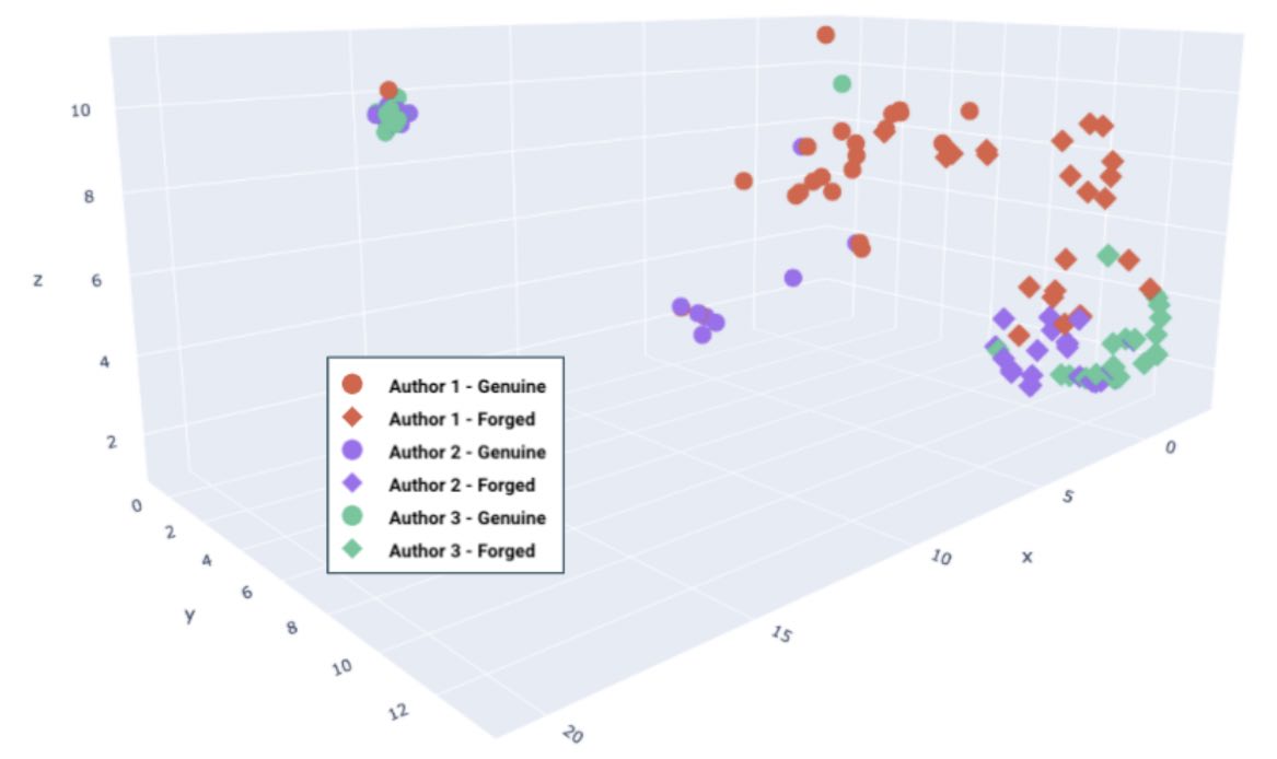
Figure 11. A 3D plot of embeddings produced by a network trained with contrastive loss, for three authors’ signatures. Genuine vs. forged examples are appropriately placed into separable regions, as seen by groupings of circles vs. diamonds.
Second, contrastive loss is limited in its ability to learn global, contextual feature representations. Figure 11 above depicts embeddings generated from the trained Siamese network for genuine and forged signature examples from three authors. We observe that the network has correctly separated genuine vs. forged examples into separate regions, which is precisely what contrastive loss aims to accomplish. However, the model has not captured the relative similarity of signatures from the same author (which can hurt generalization to new signature datasets). Ideally, we desire a model that produces embeddings that are separable across authors and discriminative between genuine/forged classes. For example, we would like to see that all signatures from Author 3 appear in the same general region, and within that region, signatures maintain separation between genuine and forged. Because contrastive loss is formulated by looking only at pairs of images, it cannot preserve a contextual understanding of author classes, and simply just learns discriminative features between genuine and forged. This shortcoming is solved by triplet loss (as we will see), and therefore the remainder of our exploration focused on this superior loss function.
Triplet Loss Training and Evaluation
We constructed several model architectures (see Table 1 below) and trained them using the Triplet Semi-Hard loss implemented in the Tensorflow addons library. [5] Each model had a similar set of final layers (two conv2D layers, followed by a Dense layer and an L2 Normalization layer with size 256). We found that adding an L2 Normalization layer after our output embeddings (as suggested in [2]) was useful in constraining the embeddings to a hypersphere conducive for cosine similarity. Each model was trained with the Adam optimizer (lr=0.001), with a learning rate decay of 0.7 ever 10 steps, and trained for 25 epochs.
| Model | Description | Max Acc | EER | # Params (Million) | Size (MB) |
|---|---|---|---|---|---|
| Small ResNet50 + Skip | Initialized with weights from a pretrained ResNet50 model at layer conv4_block6_add. | 81.8 | 0.184 | 9.27 | 35.72 |
| Small ResNet50 | Initialized with weights from a pretrained ResNet50 model at layer conv4_block6_3_conv. | 76.6 | 0.236 | 9.27 | 35.7 |
| ResNet50 | Initialized with weights from a pretrained ResNet50 model. | 76.4 | 0.242 | 24.79 | 95.01 |
| Smaller ResNet50 + Skip | Initialized with weights from a pretrained ResNet50 model at layer conv3_block4_add. | 76.1 | 0.24 | 2.18 | 8.5 |
| Small ResNet50 NONORM | Initialized with weights from a pretrained ResNet50 model at layer conv4_block6_3_conv. Embedding is not L2 normalized | 75.2 | 0.249 | 9.27 | 35.7 |
| ResNet50 NONORM | Initialized with weights from a pretrained ResNet50 model. Embedding is not L2 normalized. | 75 | 0.252 | 24.79 | 95.01 |
| Pretrained VGG16 Baseline | Pretrained VGG16 without any metric learning fine tuning. | 74.3 | 0.268 | 14.71 | 56.18 |
| Small VGG16 | Initialized with weights from a pretrained VGG16 at layer block3_conv1 | 72.1 | 0.282 | 2.33 | 8.91 |
| UNet ResNet50 | UNet like model initialized with weights from a pretrained ResNet50 model at layer conv4_block6_add. | 72 | 0.281 | 9.47 | 36.61 |
| Base UNet | UNet like model. | 71.5 | 0.293 | 1.29 | 5.06 |
| Pretrained ResNet50 Baseline | Pretrained ResNet50 without any metric learning fine tuning. | 69.3 | 0.315 | 23.59 | 90.39 |
| Base CNN NONORM | CNN baseline. Embedding is not L2 normalized | 68.1 | 0.327 | 1.68 | 6.44 |
| Base CNN | CNN baseline. | 68 | 0.327 | 1.68 | 6.44 |
| VGG16 | Initialized with weights from a pretrained VGG16 model. | 67.4 | 0.328 | 15.04 | 57.42 |
Table 1. Performance for multiple models evaluated on a test set with hard negative pairs. All models are trained with the triplet loss objective (except the pretrained VGG16 and ResNet50 baseline).
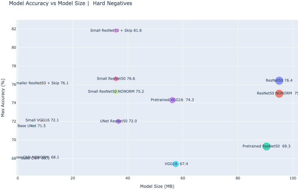
Figure 12. Maximum accuracy vs. model size for multiple model architectures, evaluated on the signature verification task.
Effect of Triplet Model Choices
Training multiple models allowed us to explore the impact of the design choices a data sciencist must navigate when applying metric learning in practice.
Impact of a Metric Loss Formulation: We see that fine-tuning a pretrained model using the triplet loss leads to a 81.8% maximum accuracy for our best model. This is a significant improvement from a pretrained ResNet50 baseline performance of 74.3%.
Impact of Pretrained Features: In our previous experiments, we saw that a pretrained model could be a strong baseline without any finetuning. To evaluate how much of the performance increase we see in our metric learning experiments is attributable to the use of pretrained features (vs. the triplet loss function), we trained a vanilla baseline CNN, as well as models constructed from intermediate layers of a pretrained ResNet and VGG16 model.
- Base CNN - 68%, 1.68 million parameters
- Base UNet - 71.5%, 1.29 million parameters
- Small ResNet50 Skip initialized at skip connection layer conv4_block6_add - 81.8%, 9.2 million parameters. (best performance)
- Smaller ResNet50 Skip initialized at skip connection layer conv3_block4_add - 76.1%, 2.18 million parameters
- Full ResNet50 fine-tuned on the triplet metric learning objective - 76.4% 24.79 million
Overall, we found the following to be useful insights:
- Fine-tuning with pretrained features (e.g., Smaller ResNet50 vs Baseline CNN and Baseline UNet) yields better results compared to training a model from scratch.
- A UNet-like architecture for models of comparable size yields better performance for our task (Base UNet vs Base CNN).
Impact of Skip Connections: Skip connections in CNNs have been shown to improve the loss surface 5 for deep networks, making them easier to train and yielding performance.
- Fine-tuning a full ResNet50 model (which has skip connections) achieves better performance (76.4%) compared to fine tuning a VGG16 model (67.4%).
Intermediate model vs Full Model: When applying transfer learning, the data scientist must decide how much of the pretrained model is useful to their task - i.e., what features to include, what features to freeze, and what features to finetune.
- We found that we got the best performance when we constructed an intermediate model from ResNet50 (Small ResNet50 skip, 35MB) and fine-tuned it, vs. fine-tuning the entire ResNet50.
- Furthermore, we found that when we constructed this intermediate model using the output of a skip connection vs. a conv2D layer, the results were better. Our intuition is that the later layers in a pretrained ResNet50 model contain high level features (e.g., eyes, wheels, doors) that are not relevant to our task and dataset (which are mostly lines and texture in a signature) and can introduce noise. More importantly, an intermediate model is faster to train, significantly smaller, and hence easier to deploy (e.g., as a microservice with limits on file sizes). Note that Smaller ResNet50 is competitive (76.1% on hard negatives, 95% on easy negatives), but only 8.5mb in file size.
Notes on training with triplet loss:
- Ensure a large enough batch size is selected when training with the online triplet loss (on the minimum, batch size should be greater than the number of classes). This ensures each batch contains enough samples such that a valid semi-hard triplet can be sampled. A NaN loss value during training might indicate that your current batch size is too small.
- Ensure the distance metric used in the loss function is the same distance metric that will be used during evaluation/test time. (E.g., if cosine distance is used in the loss function during training, it should also be used when comparing the similarity of two signatures at test time. For example, a model trained with an L2 distance function will show reduced accuracy when evaluated with cosine distance.)
- Modifying the margin parameter can be used to improve the performance of each model. (For example, if loss does not decrease during training, it might indicate that it is challenging to find good triplets (e.g., negatives are too hard and yield similar embeddings); in this case, decreasing the margin parameter can be useful.)
Debugging a Metric Learning Model - Does It Do What We Think It Does?
So far, we have built several models with competitive results. However, it is important to verify that the model is in fact achieving its goals (similar signatures close together, dissimilar signatures far apart), and that it is doing this for the right reasons.
To this end, we explored several sanity check approaches to help us build trust and confidence in the model’s behaviour. Sanity checks help us confirm expected behaviours and question any unexpected or unusual observations.
Dimensionality Reduction + Visualization
First, we have used dimensionality reduction techniques (UMAP) to visualize embeddings for each signature in our test set. We expect that signatures from the same author are clustered together; we also expect that skilled forgeries are close to originals, but separated from the cluster of the associated genuine signature.
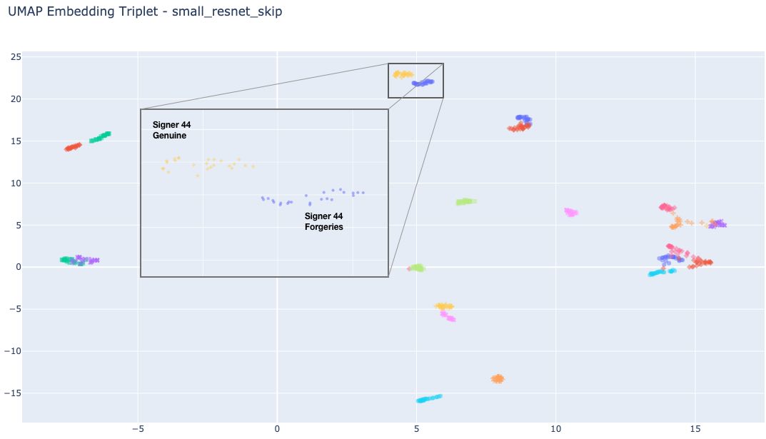
Figure 13. Visualization of UMAP embeddings (2 dimensions) for signatures in our test set. In general, we see that embeddings for forgeries are in the same region as their corresponding genuine signatures, but still separated.
Visualization of distance metrics
In this sanity check, we construct image pairs (positive and negative pairs) and compute the distance between embeddings produced by our model for each pair. We expect that the density of distances between positive pairs is close to zero (with some variation to account for user error), but more spread out toward 1 for negative pairs.
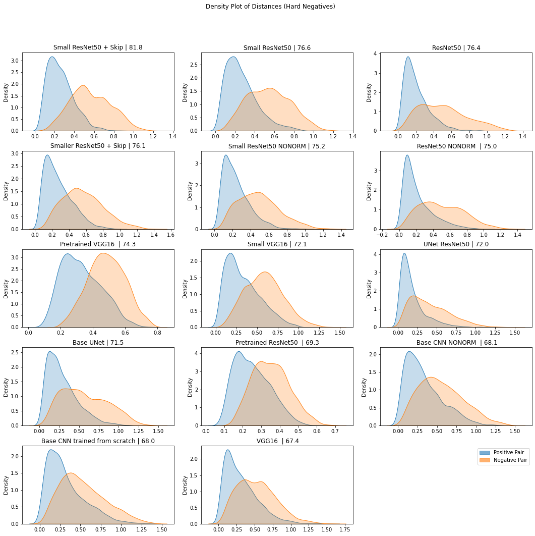
Figure 14. Density plot of the cosine distances between embeddings (produced by multiple models) for positive and hard negative pairs in our test set.
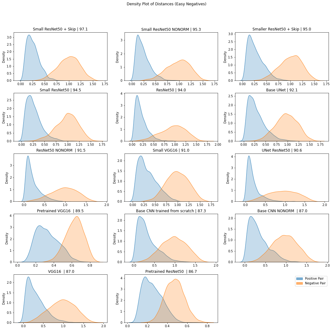
Figure 15. Density plot of the cosine distances between embeddings (produced by multiple models) for positive and easy negative pairs in our test set.
Gradient Visualization of Class Activation Maps
We can also utilize gradient based approaches 6 to inspect “what aspects of the input are most influential/relevant to the output.” These approaches have been used in debugging classification models to identify what pixels in the input image drive a specific class prediction. For example, we want to see that pixels around the head and ears of a husky dog are the relevant regions, as opposed to a snow background, when predicting the husky class. A well-known approach in this area is GradCam, 7 which visualizes the gradient of the class score (logit) with respect to the feature map of the last convolutional unit of a DNN model. We can adapt it to our use case by visualizing the gradient of the entire output embedding with respect to the feature map of a preselected convolutional layer in our metric learning model. What this visualization gives us is some intuition on the region within the input signature that our layer finds influential while producing embeddings. Ideally, we want to see a concentration around the actual lines and strokes of the signature, and possible focus on parts of written letters that might have high variance (e.g., attention to how users might round their g’s in a unique way). Our implementation of GradCam is based on the Keras GradCam example here.8
Note, that methods like GradCam are not exactly principled, but subject to interpretation based on domain knowledge. The reader is encouraged to explore GradCam visualizations to confirm that the pixels which the model finds influential make sense, based on their knowledge of the problem space.
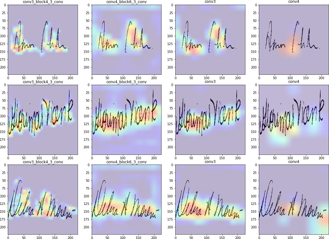
Figure 16: GradCam visualization for the last 4 convolutional layers for signatures from our test set.
Limitations
In this work, we’ve shown that fine-tuning a pretrained model on a metric learning loss (contrastive and triplet loss) can improve performance. However, there are a few limitations with our experiment’s setup that are worth noting:
-
Dataset Limitations: While our training setup is designed such that we evaluated the models on signatures from individuals not represented in the training set, we recognize that the CEDAR dataset is small, and does not cover properties of signatures (e.g., different writing styles, languages, etc.) that may occur in real world documents, but are not covered in the CEDAR dataset. Training and evaluation on additional datasets is strongly recommended prior to production use.
-
Limitations of Triplet Loss: While triplet loss is great, its application is limited to scenarios where labels exist. To implement intelligent construction of triplets (especially semi-hard negatives), we need labels for each class. On the other hand, we can still apply contrastive loss to unlabelled datasets by leveraging pseudo-labels (e.g., existing research 9 shows that k-means assignments can be used as pseudo-labels to learn visual representations).
-
Data Augmentation: We used the CEDAR dataset as is, without exploring augmentations or transformations. For example, it may be useful to experiment with scale or rotation transforms, to ensure the model is invariant to these changes.
-
Reproducibility: Deep Neural Networks can have multiple sources of randomness, which can make it challenging to reproduce the exact results we report. These may include hardware properties, weight initialization, etc. In our experiments, we attempted to minimize this by fixing the seeds for numpy and tensorflow. We still observed slight variations across each run (~3 percentage points) - however, the relative order of results stayed consistent.
-
Model Tuning: In our experiments, while we explored the impact of metric loss finetuning, pretrained features, and skip connections over a small set of presets, there are still many parameters that can be tuned. These include margin parameter, learning rate, model architecture (e.g., use of models designed to learn multiscale features), etc.
-
Other Loss Functions: While we have focused on contrastive and triplet loss, there are other valid (and perhaps less complicated) ways of fine-tuning a pretrained model that yield good distance metrics. For example, we could explore a cross-entropy loss that learns to predict a class (genuine, skilled forgery, unskilled forgery), given a pair of images. (The reader is encouraged to review the work of Boudiaf, Malik, et al. for further insight on how cross-entropy loss compares with other metric learning losses.) 10
Naturally, these limitations are opportunities for future work and experiments.
Summary and Conclusion
Metric learning helps us train a model that yields representations of similarity adapted to our task and dataset. In this post, we have covered several loss functions for metric learning (contrastive loss, triplet loss, quadruplet loss, and group loss). We also reported on a set of experiments training a model for signature verification on the CEDAR dataset.
We learned that:
- Pretrained models can be strong baselines for the signature verification task. When the problem is easy (i.e., unskilled forgery), we see that a pretrained VGG16 model yields 89.5% accuracy and 74.3% when the problem is hard (skilled forgeries).
- Triplet loss achieves better performance compared to contrastive loss, and learns a better overall structure of the embedding space.
- Triplet loss (with online triplet mining) is more efficient to train, compared to contrastive loss (i.e., training time to reach maximum accuracy). It does not require the manual construction of training triplets (as required in contrastive loss) and uses intelligent sampling to select informative triplets. This is very useful when running experiments to explore a large hyperparameter space. As an example, we found that finetuning a ResNet50 model with triplet loss was completed in three minutes, while a contrastive loss model needed eight hours to reach max accuracy.
- With respect to implementation, we found the Tensorflow addons implementation of triplet loss 11 to be useful.
- Fine-tuning an intermediate model can not only result in a reduced model size, but also improved accuracy. Our experiments suggest that for the task of signature verification, fine-tuning a subset of the ResNet50 model resulted in a smaller model size, compared to fine-tuning the entire ResNet50 model.
- A good practice is to use the same distance metric across training and test. L2 distance is more computationally efficient compared to cosine distance, making it the better choice in production. L2 similarity measures are also well-supported by libraries designed for fast approximate nearest neighbor search (e.g., Annoy, FAISS, ScaNN). Also note that computing L2 distance on normalized embeddings (recall our L2 normalization layer earlier) yields the equivalent of cosine distance.
References
-
Understanding Ranking Loss, Contrastive Loss, Margin Loss, Triplet Loss, Hinge Loss and all those confusing names. https://gombru.github.io/2019/04/03/ranking_loss/ ↩︎
-
Schroff, Florian, Dmitry Kalenichenko, and James Philbin. “Facenet: A unified embedding for face recognition and clustering.” Proceedings of the IEEE conference on computer vision and pattern recognition. 2015. ↩︎
-
Chen, Weihua, et al. “Beyond triplet loss: a deep quadruplet network for person re-identification.” Proceedings of the IEEE conference on computer vision and pattern recognition. 2017. ↩︎
-
Elezi, Ismail, et al. “The group loss for deep metric learning.” European Conference on Computer Vision. Springer, Cham, 2020. ↩︎
-
Li H, Xu Z, Taylor G, Studer C, Goldstein T. Visualizing the loss landscape of neural nets. arXiv preprint arXiv:1712.09913. 2017 Dec 28. ↩︎
-
Adebayo, J., Gilmer, J., Muelly, M., Goodfellow, I., Hardt, M., & Kim, B. (2018). Sanity checks for saliency maps. arXiv preprint arXiv:1810.03292. ↩︎
-
Selvaraju, Ramprasaath R., et al. “Grad-cam: Visual explanations from deep networks via gradient-based localization.” Proceedings of the IEEE international conference on computer vision. 2017. ↩︎
-
Grad-CAM class activation visualization https://keras.io/examples/vision/grad_cam/ ↩︎
-
Caron, Mathilde, et al. “Deep clustering for unsupervised learning of visual features.” Proceedings of the European Conference on Computer Vision (ECCV). 2018. ↩︎
-
Boudiaf, Malik, et al. “A unifying mutual information view of metric learning: cross-entropy vs. pairwise losses.” European Conference on Computer Vision. Springer, Cham, 2020. ↩︎
-
TensorFlow Addons Losses: TripletSemiHardLoss https://www.tensorflow.org/addons/tutorials/losses_triplet ↩︎