Jan 31, 2022 · post

Why and How Convolutions Work for Video Classification

Video classification is perhaps the simplest and most fundamental of the tasks in the field of video understanding. In this blog post, we’ll take a deep dive into why and how convolutions work for video classification. Our goal is to help the reader develop an intuition about the relationship between space (the image part of video) and time (the sequence part of video), and pave the way to a deep understanding of video classification algorithms.

To accomplish this goal, we will take the following approach

• Preliminaries: description of the video classification task, the types of approaches to video understanding, general aspects of convolutions, and notation used in the rest of the post.
• Why and How Convolutional Neural Networks Work: discussion of spatio-temporal hierarchical features, and spatio-temporal invariance.
• Space-time Anisotropy: explanation of why spatial directions are treated similarly in convolutional networks, why time is treated differently, and what that all means for the design of video classification architectures.
• Summary: a synopsis of the three main takeaways from this blog post.

Related blog: For a broad and introductory view of the field of video understanding please see our previous blog post, in which we discuss the many tasks associated with this field, including video classification, as well as their applications in the real world.

Related code: Concurrent with the publication of this blog post, Cloudera Fast Forward Labs is also releasing an applied prototype focused on video classification.

Preliminaries

In this section, we describe the machine learning task of video classification, provide a brief taxonomy of video classification methods, explain general aspects of convolutions, and describe the notation used in the rest of the post.

The Video Classification Task

Video classification is similar to other classification tasks, in that one item is used as input to a predictive model, and one set of scores is produced as output. For video classification, as illustrated in Figure 1, the input is a video clip, and the output is typically a set of action class scores. In a way, video classification is analogous to image classification, but instead of detecting what kind of object is present in an image, video classification is used to detect what kind of action is happening in a video.

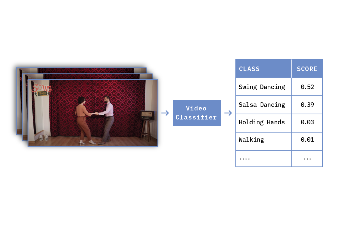Figure 1. Illustration of Video Classification. On the left is the video clip being classified, and on the right are human action classes. Scores measure how likely it is that the action is performed at any time during the video. The images on the left were taken from a YouTube video (part of the Kinetics 400 dataset).

Approaches to Video Classification

As in many other areas of machine learning, the most exciting developments in video classification involve the use of deep neural networks (DNN). DNN-based approaches can be divided into three categories, depending on the type of operations used: convolutions, non-local operations (like attention), or hybrid.

The use of convolutions in video classification is motivated by the fact that they have been shown to excel at extracting features from images, and video consists of images. The use of non-local operations, on the other hand, has different motivations. For example, a non-local operation like attention is highly effective for processing sequences, and video is a sequence. Additionally, from the perspective of classical (non-deep learning) computer vision, non-local approaches like non-local means have been successfully applied in computer vision for years — long before the current deep learning era.

This blog post focuses on convolutions, for three reasons. First, convolutions still dominate the computer vision landscape, in spite of recent progress in attention-based methods. Second, even if non-local approaches become dominant in the near future, having a thorough understanding of why convolutions work for video paves the way to an understanding of why non-local approaches work, too. Third, it is plausible that convolutions and non-local approaches are complementary, as argued in this article.

Convolutions: General Aspects

Convolutions are perhaps the most widely used operation in the deep-learning era of computer vision. They are powerful feature extractors, they present useful properties like translational invariance, and they help reduce the number of parameters when compared, e.g., with fully connected layers. Convolutional neural networks (CNNs) are built by stacking layers of convolutions, each typically followed by non-linear and pooling operations. Sequences of layers are capable of hierarchically building rich features.

Notation

Throughout the rest of this blog post, the shapes of tensors holding feature maps and convolutional kernels will be denoted by 4-tuples: (Length, Height, Width, Channels), where

• Length = temporal length. When the feature map is a video, Length corresponds to the number of frames in the video. When the map is a still image, Length=1. Length is the temporal dimension of the feature map.
• Height = height of the video frames. This is one of the two spatial dimensions.
• Width = width of the video frames. This is the other spatial dimension.
• Channels = number of color channels. This is the color dimension.

Figure 2 illustrates a generic tensor and its dimensions.

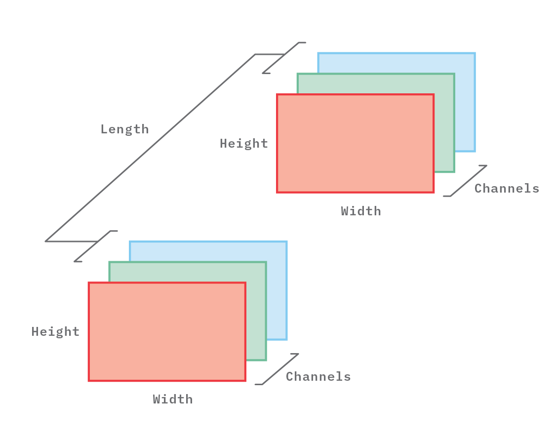Figure 2. Illustration of a 4-dimensional tensor, with shape (Length=2, Height, Width, Channels=3).

In the following discussion, we use images and videos as the input maps, but the same ideas apply when the inputs are features produced by inner layers of a CNN, e.g, activations of convolutions from previous layers, or pooling operators.

Why and how CNNs work for video

In this section, we will first describe 2D convolutions applied to grayscale images, and then 3D convolutions applied to grayscale video. The third and fourth subsections present the color counterparts of the first two. The color cases are presented for completeness, and also to make clear the distinction between color channels and temporal channels. (The second subsection contains the main takeaways, though, so if you have time to read only one subsection, that should be it!)

Grayscale Images

Figure 3 illustrates a 2D convolution applied to a grayscale image. Grayscale images have one color channel only. The image, or input feature map, has shape (1, H, W, 1), the convolutional kernel has shape (1, h, w, 1), and the output feature map has shape (1, H’, W’, 1). The output spatial dimensions H’ and W’ depend on the type of padding (same, valid, etc.) and on the stride size (the size of the ‘jumps’ that the kernel makes as it is moved across the input data). In all that follows, we will assume valid padding and stride=1 in all dimensions, although this detail is not central to the main takeaways.

The kernel spatial dimensions are typically smaller than the image spatial dimensions: h < H and w < W; this is what makes the operation local. Also, the kernel is typically applied multiple times, in a sliding fashion, through the input map. Each time the kernel is applied, a new point is produced in the output map. In this way, the kernel can be said to be striding along two dimensions: namely, along the height and along the width of the input image. Those two directions are shown in Figure 3 as arrows inside the input feature map, and are what make the convolution two-dimensional. The label t=1 refers to the fact that only one moment in time is considered, as it is an image, rather than a video.

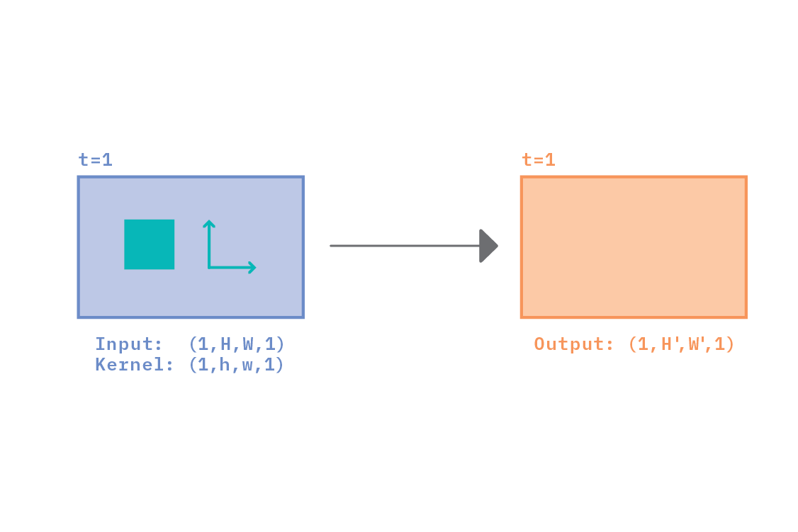Figure 3. Illustration of a 2D convolution applied to a single-channel input feature map, e.g., a grayscale image. The kernel can only stride in two dimensions (vertically and horizontally, denoted by small arrows), which is why the convolution is termed two-dimensional.

Because the kernel maintains fixed parameters as it strides, convolutions are said to be translationally invariant (this is not the case in operators like attention). Invariance gives convolutions the capability to detect the same structure (e.g. an edge, corner, etc) anywhere in the input map. At each location in the map, the kernel gathers information within a limited spatial region, which makes the operation local (again, this is not the case in the attention mechanism).

Subsequent layers in a convolutional neural network (CNN) apply convolutions on maps produced by previous layers, which (in addition to convolutions) can involve, non-linear activations and pooling operations. In this way, increasingly complex structures (such as those corresponding to objects in the case of object detection) can be detected.

Grayscale Video

Figure 4 illustrates a 3D convolution applied to a very short grayscale video of length L=4. Individual frames are labeled t=1,2,3,4, corresponding to four different points in time in the video.

The convolutional kernel in the figure has been chosen to have shape (l=2, h, w, c=1). Just as the spatial dimension of the kernel is typically smaller than the spatial dimension of the feature map (h < H, and w < W), the temporal dimension of the kernel (l=2 in the example) is also typically smaller than the temporal dimension of the input map (L=4 in the example).

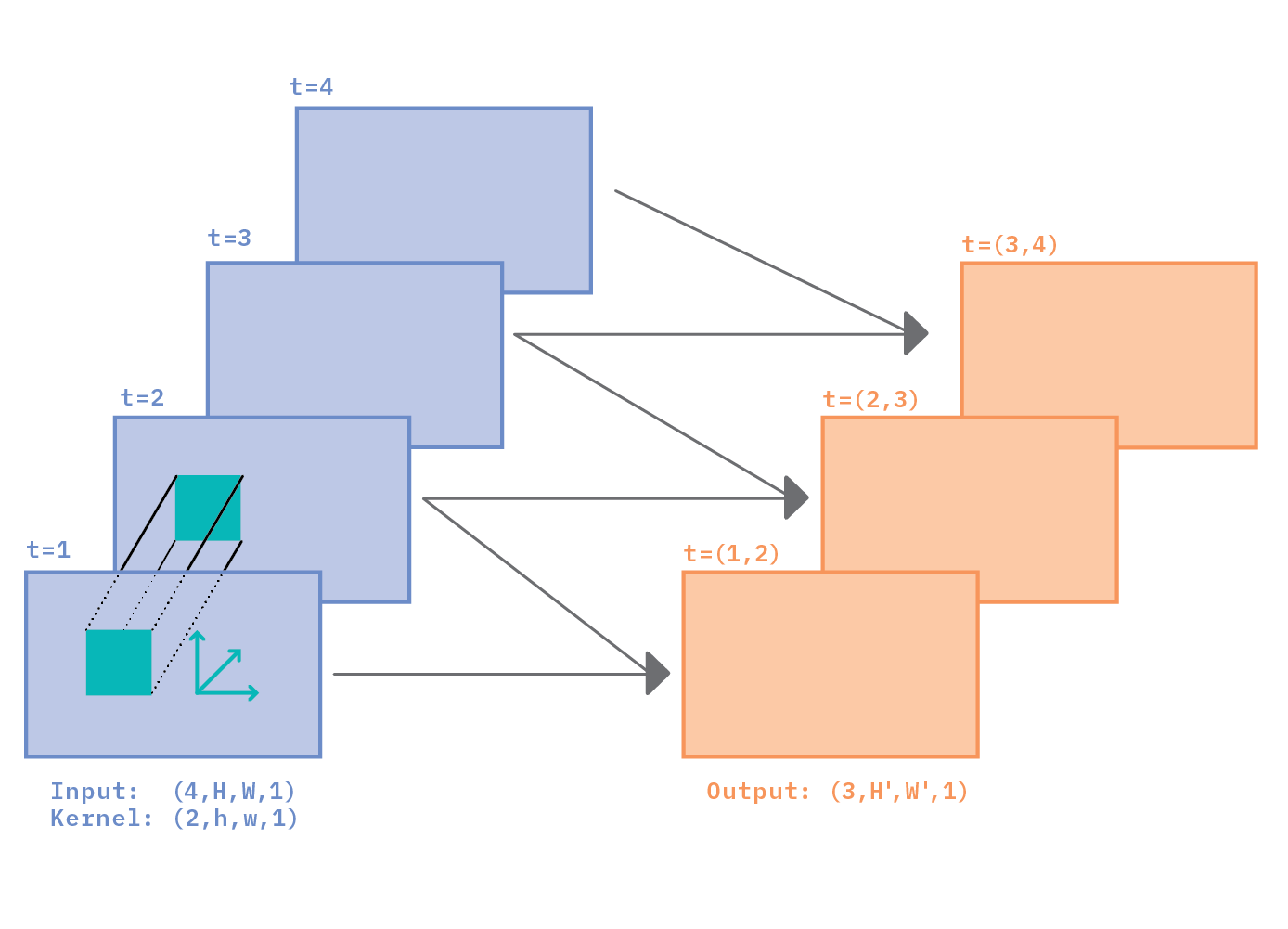Figure 4. 3D convolution applied to a grayscale video with four frames. The kernel is strided along three dimensions: vertical, horizontal, and temporal.

In order to extract information from the full video, a kernel now has to stride across three dimensions: two spatial, and one temporal. Striding along spatial dimensions produces neighboring points on the same output feature map. Striding along the temporal dimension produces points on different output feature maps.

Because we have chosen the temporal length of the kernel l=2 in Figure 4, there can only be three output feature maps, each of which contains information about pairs of consecutive input frames. This is indicated by labels t=(1,2) for the first output map, t=(2,3) for the second map, and t=(3,4) for the third map.

Takeaway 1: Spatio-Temporal Hierarchical Features

We now point to a contrast and a similarity between 2D and 3D convolutions:

• In contrast with 2D convolutions, where the output map contains information only about the spatial variations in the input, 3D convolutions collect information about both spatial and temporal variations.
• In the same way as complex spatial information is built across multiple 2D convolutional layers of a CNN (which have the capability to, e.g., detect objects), complex spatio-temporal information is also built across multiple 3D layers (which have the capability, e.g., to detect actions). The different levels of complexity across layers of a CNN is often referred to as a hierarchy of features.

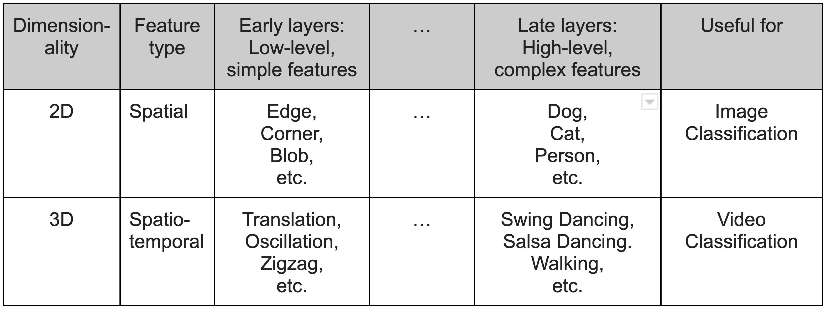Table 1. The complexity of features in early and late layers for 2D and 3D convolutions.

Table 1 shows the idea of going from simple, low-level features in the early layers of a CNN to the complex, high-level features of late layers — both for 2D and 3D. For 2D, the features go from simple structures (like edges, corners, or blobs) to ultimately complex object structures (like the shape of a dog, cat, or person). This is useful for image classification. In the 3D case, the features are spatio-temporal, and may in the early layers include basic types of motion (such as translation, oscillations, zigzag, etc.) Later layers would produce complex motion features (such as those that help distinguish swing dancing from salsa dancing). The spatio-temporal aspect comes from the fact that, in order to distinguish an action from another, it might be necessary to know both the what (a hand, the head, or the hips of a person) as well as the how (up and down, sideways, etc.)

Let’s see how hierarchy impacts architectural design aspects. In Figure 4, had we chosen a temporal kernel length l=3 rather than l=2, information would have been gathered from three consecutive frames instead of two. The l=3 case is illustrated in Figure 5.

Figure 5. Similar to Figure 4, but with a larger kernel length along the temporal dimension (l=3).

Larger temporal sizes for the kernel could, at first, seem better than smaller sizes: after all, actions tend to be more discernible when we look at more than two consecutive frames (a small fraction of a second in a video running at 25 frames per second).

However, as mentioned above, deep CNNs are meant to build features gradually, from short scales (both temporally and spatially) in the first few layers, to long scales in later layers. Because convolutions take a (weighted) average of feature values, having kernels that are too large results in the loss of fine-grained information. On the other hand, having relatively small kernels helps to capture actions that occur on short time scales (e.g., to detect clapping, which may happen, say, on the order of 0.5 seconds). It is the many layers that allow CNNs to gradually build features describing long time scale actions (e.g., swing dancing, which may require several seconds for it to be discernible from, say, salsa dancing) from short scale, atomic motion features. Striking the optimal size of kernels is one of the challenges that CNN designers face.

Takeaway 2: Spatio-Temporal Invariance

In the same way as 2D convolutions have built-in invariance in space, 3D convolutions have invariance in time.

• 2D translational invariance results in convolutions being able to detect objects anywhere in space, which is helpful in image classification, because it doesn’t matter where the object is located.
• 3D translational invariance results in the capability to detect actions at any point in time, which is useful for video classification, where it is not important when the action is happening.

We will expand on those insights in later sections, but first we will present the case of color images and video. Conceptually, there is no significant difference between grayscale and color, but for practical purposes (e.g., when specifying the shapes of tensors in code), it is useful to have clarity on the difference between the temporal dimension and the color dimension.

Color Images

Figure 6 illustrates a 2D convolution applied to a color image. The input shape is (1, H, W, 3): the 1 corresponds to the single frame (a still image rather than a video), and the 3 is for the three 3 color channels (e.g., corresponding to an RGB image). The convolutional kernel has shape (1, h, w, 3). In spite of both tensors (input image and kernel) having three color channels, the kernel is only strided across the two dimensions, which makes the convolution 2D. The output has shape (1, H’, W’, 1), which means that each output feature point has information from all the three channels of a small spatial region in the input.

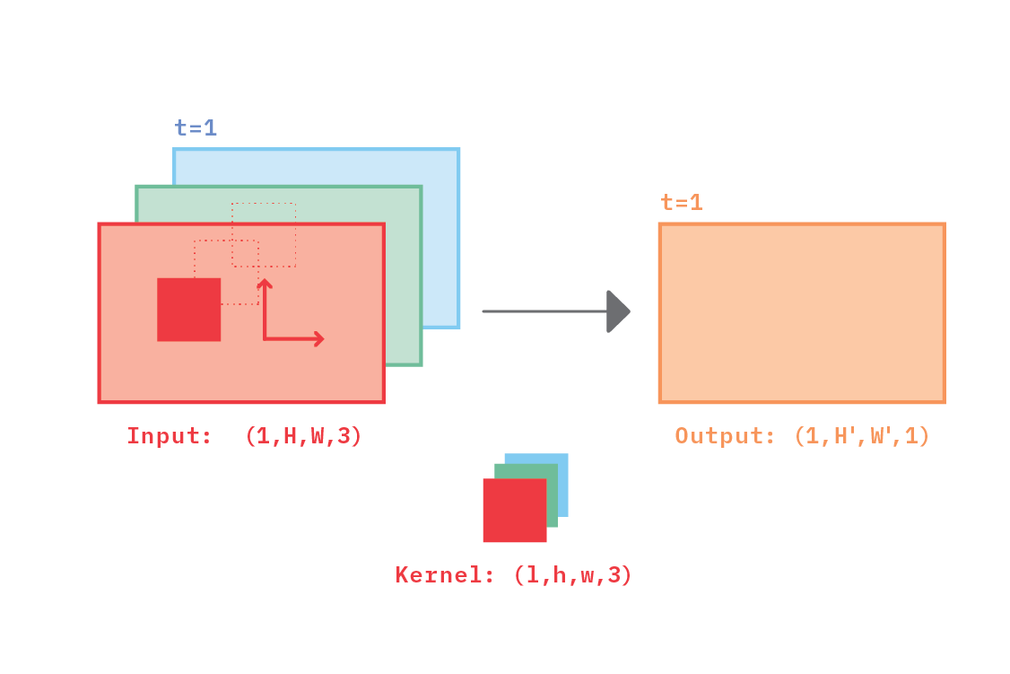Figure 6. A 2D convolution applied to a color image. Both the input feature map and the kernel have three color channels, but the kernel is only strided along two dimensions: vertically and horizontally.

Color Video

Figure 7 illustrates the case of a 3D convolution applied to a very short color video containing four frames. The shape of the input is (4, H, W, 3), with 4 frames of 3 color channels each. The frames are labeled t=1, 2, 3, 4, corresponding to the four points in time captured in the video. The convolutional kernel has shape (2, h, w, 3).

We can see in Figure 7 that for the kernel to collect information from all of the video, it has to be strided along three directions: two spatial, and one temporal. Every time the kernel is applied at one location (in space-time) of the input, information is collected from all three channels of two consecutive frames.

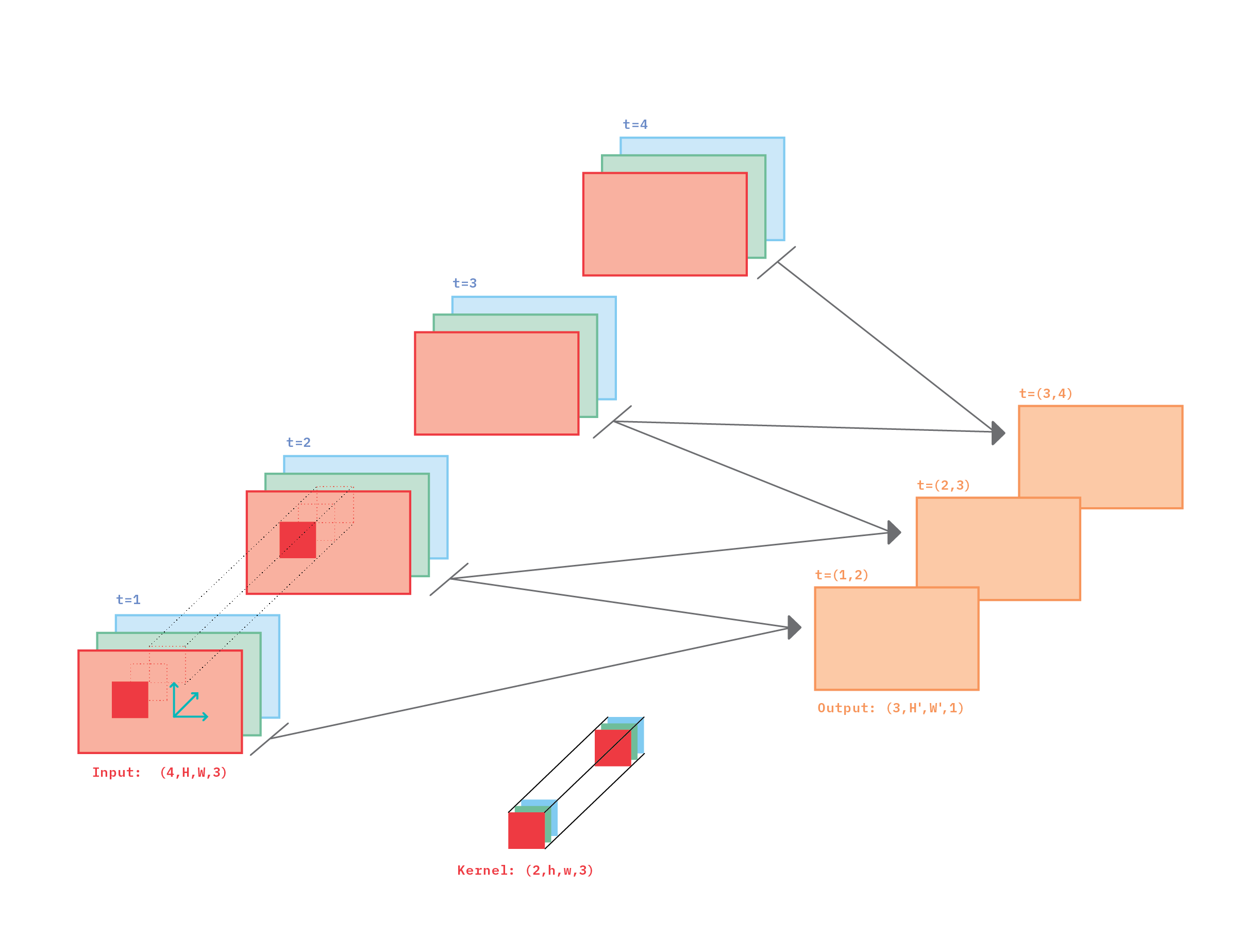Figure 7. A 3D convolution applied to a short color video with four frames. The color of the video is encoded in three channels (e.g., RGB format).

The intuition behind color video is essentially the same as for grayscale video: information is gathered from frames that are next to each other in time, and complex motion features are built when multiple layers are traversed in a CNN.

Space-Time Anisotropy

There is one more concept in video data which we’d like to discuss: anisotropy. By “anisotropy” we mean a change in the properties of a system when they are measured along different axes. In our case the axes are those of the tensors holding feature maps and convolutional kernels. Though not explicitly, we have already touched upon this concept, in the [Spatio-Temporal Hierarchical Features](#Spatio-Temporal-Hierarchical Features) subsection. Here, we take a deeper dive.

To better understand the idea, it is useful to review the concept of receptive field.

Receptive Field

The receptive field of a feature (in a neural network) is the size of the region in the input (to the network, not the layer) that influences the value of that feature. Figure 8 illustrates the concept of a receptive field for a two-layer CNN, where the convolutions are 2D. Each feature in Layer 1 is influenced by a 3x3 region of the input feature map (in blue). However, in Layer 2, each feature is influenced by a region of size 5x5 in the input feature map (in blue and in gray).

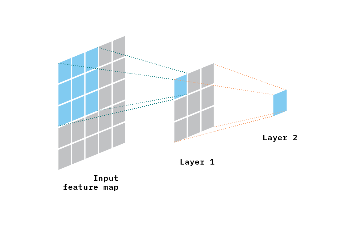Figure 8. Illustration of the concept of receptive field. Layer 1 has a receptive field of size 3x3. Layer 2 has a receptive field of size 5x5 (all of the input layer).

Generally speaking, the deeper the layer, the larger the receptive field. This is so because every convolution combines features which were themselves a combination of features in earlier layers. For image classification, for instance, the field of view eventually covers the full image, as the output (e.g., the score assigned to each class) should depend on the full image.

Figure 9 illustrates the idea of a temporal receptive field for 3D convolutions. The temporal receptive field is the number of frames in the input feature map (the first column of frames, on the left of the figure) that influences a feature in a given layer. After convolution 1, there are three feature maps; feature points on each of those maps are influenced by two frames [t=(1,2), t=(2,3), or t=(3,4), respectively]. After convolution 2, there are two maps, and feature points on each of them are influenced by three frames [e.g., t=(1,2,3), and t=(2,3,4)]. After convolution 3, there is only one map; each feature in that map is influenced by all four input frames [t=(1,2,3,4)]. In this artificial example, features in the last layer have “looked” at all of the input frames, and could, in principle, detect an action anywhere in the video.

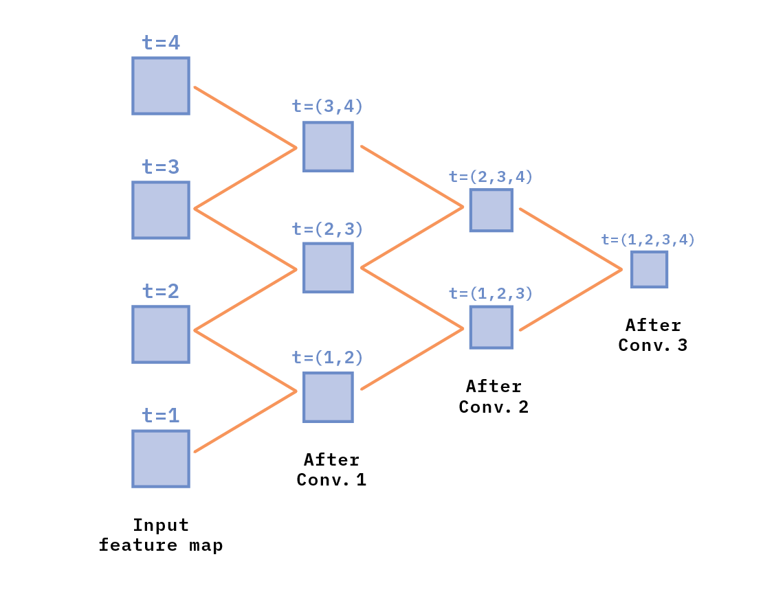Figure 9. Illustration of the concept of temporal field of view.

With this understanding of the concept of spatial and temporal receptive fields, let’s dive into the idea of space-time anisotropy.

Takeaway 3: Space-Time Anisotropy

When performing image classification, it makes sense that the two spatial dimensions (vertical and horizontal) are treated equally: vertical and horizontal distances in a feature map should count with equal weight. This feature helps detection of objects regardless of their orientation, and is achieved by setting the vertical and horizontal size of the convolutional kernels to the same value. Similarly, the stride size is typically the same vertically and horizontally. We can think about this as some kind of isotropy encoded in the architectural choices.

But what happens when we go from 2D to 3D convolutions, which have a temporal dimension? Time differs from space. Therefore, there is no reason for the sizes of a convolutional kernel and stride to necessarily have the same size temporally as spatially.

This is illustrated in Figure 10, where a 3D convolutional kernel is depicted. It has spatial size w=h=3, and temporal size l=4.

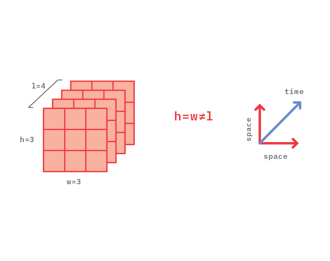Figure 10. Illustration of a kernel that has the same spatial size horizontally and vertically (h=w=3), but different size temporally (l=4).

As an example, let’s consider the case of a 2D CNN for object detection. Let us further say that one of the classes to be detected is a pair of hands. This might be achieved by having a layer, deep in the network, with a spatial field of view of, say 300 pixels vertically and 300 pixels horizontally (assuming that’s the size of the hands in the input image). This would allow the detector to find hands, regardless of their orientation.

Let’s now consider the case of a 3D CNN for video classification, and that one of the classes to be detected is “clapping hands.” To that end, the CNN might include a layer with a temporal field of view of, say, 25 frames (or 1 second, if the input video has a frame rate of 25 frames per second). In this case, the optimal field of view for the layer that detects clapping hands might be on the order of 25x300x300 (where the first number is the temporal size, and the remaining two numbers are the spatial size), which manifests the anisotropy in time-space.

Summary

We hope the ideas presented in this blog post will help the reader develop an intuition about why and how convolutions work for video classification. To summarize, here are our three main takeaways:

1. Hierarchical features (increasing levels of complexity as one moves from early to late layers in CNNs) helps explain both 2D and 3D CNNs. In 2D CNNs, features are spatial, and represent increasingly complex shapes, which eventually help identify objects in images. In 3D CNNs, the features are spatio-temporal, and represent increasingly complex shapes-motion, which eventually help identify actions in video.
2. Translational invariance of 2D convolutions allows recognition of objects in images regardless of their position in space, whereas invariance in 3D convolutions allows recognition of actions in video regardless of their location in time or space.
3. Space-time anisotropy is related to the fact that space differs from time, which has implications for CNN design.

Resources

These are some of the articles that influenced the content of this blog post:

• Learning Spatiotemporal Features with 3D Convolutional Networks, Tran et al., 2014 (updated 2015).
• Spatiotemporal Residual Networks for Video Action Recognition, Feichtenhofer et al., 2016.
• Quo Vadis, Action Recognition? A New Model and the Kinetics Dataset, Carreira and Zisserman, 2017.
• Non-local Neural Networks, Wang et al. 2018.
• Is Space-Time Attention All You Need for Video Understanding? Bertasius et al., 2021.