Jul 11, 2022 · post

Automated Metrics for Evaluating Text Style Transfer

By Andrew Reed and Melanie Beck

In our previous blog post, we took an in-depth look at how to neutralize subjectivity bias in text using HuggingFace transformers. Specifically, we saw how to fine-tune a conditional language model (BART-base) on the Wiki Neutrality Corpus (WNC) and benchmarked its performance against the WNC paper authors’ modeling approach on a subset of the dataset which only included one-word edits.

In this post, we’ve expanded our modeling efforts to the full dataset consisting of ~180,000 subjective-to-neutral sentence pairs. These pairs include the one-word edits that we used before, as well as all the sentence pairs with more than one-word edits – a materialy more difficult generative modeling task. We apply the same data preprocessing steps and model training configuration as discussed in the previous blog, and also propose a set of custom automated evaluation metrics aimed to better quantify the subtleties of text style transfer than traditional metrics.

Challenges with Evaluating Text Style Transfer

Evaluating the quality of machine generated text is hard. Human evaluation is regarded as the best indicator of quality, but unfortunately is expensive, slow, and lacks reproducibility, making it a cumbersome approach for validating model performance. For this reason, NLP practitioners often rely on automated evaluation metrics to serve as a cheap and quick proxy for human judgment. Of course, this compromise comes with tradeoffs.

Traditional automated metrics like the BLEU score – the most common metric for evaluating neural machine translation (NMT) – work by counting the lexical n-gram overlap between generated outputs and human-annotated, gold-standard references. As we saw in the previous blog post, BLEU is one of the metrics used by the WNC paper authors to benchmark their model performance against a set of references. Consider the task of comparing the following candidate sentence with the two references while evaluating for semantic equivalence.

Candidate: He is a great singer.

Reference #1: He sings really well.

Reference #2: He is a great writer.

As humans, it’s obvious that Reference #1 means basically the same thing as the Candidate, while Reference #2 changes the entire semantic meaning. However, because BLEU score only measures counts of identical n-grams, Reference #2 actually scores higher than Reference #1 by this metric. This highlights one of BLEU’s [many] shortcomings in that it fails to robustly match paraphrases, which leads to performance underestimation as semantically-correct phrases are penalized because they differ in lexical form¹.

While it’s clear that the BLEU metric itself is flawed, the broader “candidate-to-reference” based NMT evaluation strategy itself also poses issues for evaluating text style transfer. That’s because style transfer is a one-to-many task, which means that there are several suitable references for any one source sentence². Therefore, a high-quality style transfer generation may have a low BLEU score towards a reference as we saw in the previous example. Rather than relying on gold references, reference-free evaluation methods have been found to better align with human judgements in the analogous task of paraphrase generation.

In this reference-free paradigm, we ignore ground-truth annotations and compare model output directly with model input. Let’s now consider the scenario wherein we feed the sentence “He is a great singer.” to our text style transfer model to which it produces an output of “He is a great writer.” The first thing we notice is the subjectivity in the sentence has not been neutralized (evidenced by the word “great” in both the input and output sentences) and, worse, the very meaning of the sentence has changed – singer and writer are not the same thing!

Unfortunately, BLEU was not designed to detect style, and as we already saw, it’s not great at assessing semantics either. We’d end up with a really high evaluation score for a really bad model! For text style transfer, a “one size” score does not fit all. We need a comprehensive approach to evaluating TST.

As discussed in our Part 1: Introduction to Text Style Transfer, a comprehensive evaluation of quality for text style transfer output should consider three criteria.

1. Style strength - To what degree does the generated text achieve the target style?
2. Content preservation- To what degree does the generated text retain the semantic meaning of the source text?
3. Fluency- To what degree does the generated text appear as if it were produced naturally by a human?

All three criteria are important in making a determination of quality. If our model transfers text from subjective to neutral tone, but omits or changes an important piece of information (e.g. a proper noun or subject), it fails to preserve the meaning of the original text. On the flip side, if the model reproduces the source text exactly as is, it would have perfect content preservation, but fail completely in style transfer. Finally, the text generation is useless if it contains all the expected tokens, but in an illegible sequence.

Automated Evaluation Metrics

In the following sections, we’ll discuss reference-free, task-specific metrics aimed at tackling the first two of these criteria while also defining our implementation and design choices.

Style Strength

A common automated method for evaluating transferred style strength involves training a classification model to distinguish between style attributes. At evaluation time, the classifier is used to determine if each style transfer output is in fact classified as the intended target style. Calculating the percentage of total text generations that achieve the target style provides a measure of style transfer strength.

While this approach serves as a strong foundation for assessing style transfer, its binary nature means that a quantifiable score only exists in aggregate. The authors of Evaluating Style Transfer for Text improve upon this idea with the realization that rather than count how many outputs achieve a target style, we can capture more nuanced differences between the style distributions of the input and output text using Earth Mover’s Distance (EMD)³. The EMD metric calculates the minimum “cost” to turn one distribution into the other. In this sense, we can interpret EMD between style class distributions (i.e. classifier output) as the intensity (or magnitude) of the style transfer. Ultimately, this metric called Style Transfer Intensity (STI) produces a score that holds meaning on a per-sample, as well as in-aggregate basis.

Implementation

Figure 1 below describes the logical workflow used in our implementation of Style Transfer Intensity.

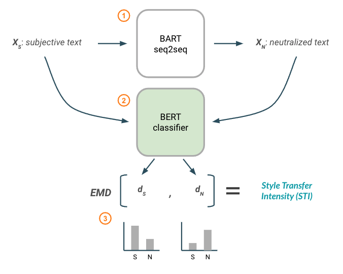Figure 1: Style Transfer Intensity metric using a BERT classification model.

First (1), a fine-tuned text style transfer model (BART) is used to generate neutralized text ( 𝑋𝑁 ) from a subjective input ( 𝑋𝑆 ). This forms the pair of text that we will be calculating the style transfer intensity between.

Then (2) both texts are passed through a fine-tuned, Transformer-based classification model (BERT) to produce a resulting style distribution for each text ( 𝑑𝑆 , 𝑑𝑁 ). These style distributions can be visualized at the bottom of Figure 1.

Finally (3), Earth Mover’s Distance is calculated on the two distributions to produce a resulting STI score. Note that like the original paper author’s, we penalize STI by negating the EMD score if the output text style distribution moves further away from the target style.

We monitor performance using accuracy as we have a perfectly balanced dataset and assign equal cost to false positives and false negatives. The best performing model produces an overall accuracy of 72.50% and has been published to the HuggingFace model registry for experimental use – please reference our training script and classifier evaluation notebook for further details.

Content Preservation

Measuring content preservation between input and output of a style transfer model is often likened to measuring document similarity. As we’ve mentioned, there are numerous techniques used to quantify similarity between text including traditional lexical-based metrics (e.g. BLEU, METEOR, ROUGE) and newer embedding-based metrics (e.g. WMD, MoverScore, SBERT). However, content preservation in the context of reference-free text style transfer evaluation is uniquely challenging. That’s because these similarity metrics fail to account for the aim of style transfer modeling, which is to alter style by necessarily changing words. Therefore, intended differences (changes in style) between source and target text are often incorrectly penalized³.

To evaluate content preservation more precisely, attempts have been made to first distinguish between semantic and stylistic components of text, and then meaningfully quantify the similarity of just the semantic component alone. While there is open debate about whether it’s possible to actually decouple style from content in free text, intuition leads us to believe that our style attribute of “subjectivity” is expressed, at least in part, through select words. For example, our EDA findings have shown that the presence of certain modifiers (adjectives and adverbs) are strong indicators of subjective content.

Previous efforts have approached this style disentanglement process by isolating just the content-related words in each sentence (i.e. masking out any style-related words). They do this by training a style classifier and inspecting the model for its most important features (i.e. words). These strong features form a style lexicon. At evaluation time, any style-related words from the lexicon that exist in the input or output texts are masked out – thus leaving behind only content-related words. These “style-free” sentences can then be compared with one of the many similarity measures to produce a content preservation score.

We draw inspiration from the aforementioned tactic of “style masking” as a means to separate style from content, but implement it in a different manner.

Implementation

Rather than construct a global style lexicon based on model-level feature importances, we dynamically calculate local, sentence-level feature importances at evaluation time. We prefer this method because the success of the Transformer architecture has shown that contextual language representations are stronger than static ones. This approach allows us to selectively mask style-related tokens depending on their function within a particular sentence (i.e. some words take on different meaning depending on how they are used in context) instead of relying on a contextually-unaware lexicon lookup.

We accomplish this by applying a popular model interpretability technique called Integrated Gradients to our fine-tuned BERT subjectivity classifier which explains a model’s prediction in terms of its features. This method produces word attributions, which are essentially importance scores for each token in a sentence that indicate how much of the prediction outcome is attributed to that token.

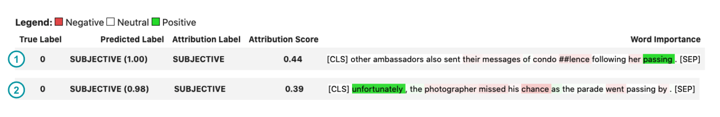Figure 2: Word attributions visualized with Transformers Interpret for two sentences using integrated gradients on the fine-tuned BERT classification model. Positive attribution numbers (green) indicate a token contributes positively towards the predicted class (“subjective”), while negative numbers (red) indicate a word contributes negatively towards the predicted class.

The figure above demonstrates the power of contextual representations. In the first sentence (1), we see that the word “passing” is strongly attributed to the subjective classification of this sentence. That’s because the term “passing” is a euphemism for “death”; a common NPOV-related correction in the WNC dataset. However, the term “passing” also appears in the second sentence (2), but is not attributed to the overall classification. That’s because the BERT model recognizes that when used in this context, “passing” does not suggest death, but rather the act of physical movement, which is neutral in tone. Had we used a global style lexicon to replace subjective words, “passing” would have been erroneously removed from the second sentence.

Provided these token level attribution scores, we must then select which are considered stylistic elements to be masked out. To do so, we sort tokens in each sentence by the absolute, normalized attribution score and calculate a cumulative sum. This vector allows us to enforce a threshold on how much of the “total style” should be masked from the sentence without having to specify an explicit number of tokens.

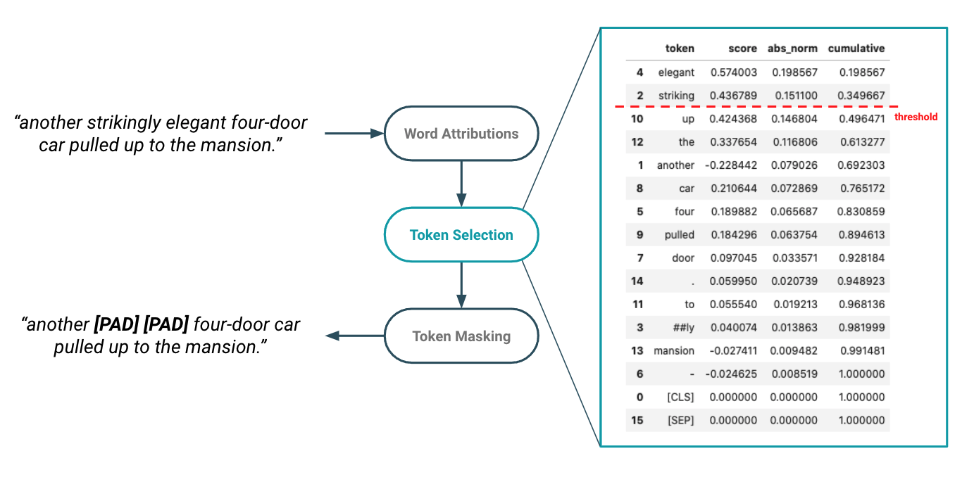Figure 3: Style masking logic determines which tokens are considered style elements and therefore masked out from the sentence prior to calculating similarity measure.

In Figure 3 above, we see how cumulative attribution scores form the basis of style token selection. In this example, the terms “elegant” and “striking” combined account for ~35% of the style classification importance. This methodology allows us to set a tunable threshold whereby we mask out all tokens that contribute to the top X% of classification importance. To “mask out” style tokens, we simply replace them with either the informationless “[PAD]” token or remove them completely by deleting in-place.

The goal of this masking activity is to create “style-independent” versions of the original input and output sentences. These style-independent texts are then encoded using a generic, pre-trained SentenceBERT model to produce sentence level embeddings. SentenceBERT is a modified version of BERT that uses siamese and triplet network structures to derive semantically meaningful sentence representations that can be compared easily using cosine similarity (see the section “To BERT or not to BERT” from our report on Few-Shot Text Classification for more on SentenceBERT). We chose this embedding-based similarity method because it overcomes the limitations of strict string matching methods (like BLEU) by comparing continuous representations rather than lexical tokens.

Figure 4 below summarizes the logical workflow used in our implementation of Content Preservation Score.

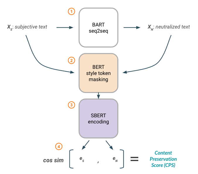Figure 4: Content Preservation Score metric using BERT-based word attributions for style masking and SentenceBERT embeddings for similarity.

To begin (1), a fine-tuned text style transfer model (BART) is used to generate neutralized text (X_N) from a subjective input (X_S) .

Style tokens are then masked from both texts (2) using the methodology described in Figure 3 above to produce versions that contain only content-related tokens.

Next (3), the content-only texts are passed through a generic, pre-trained SentenceBERT model to produce a sentence embedding for each text (e_S , e_N). Finally (4), we calculate cosine similarity between the embedding representations.

Considerations

While the high-level reasoning behind our implementations of STI and CPS make logical sense, there are nuances to the implementation that create room for error and jeopardize their effectiveness in measuring text style transfer. This is true of all automated metrics, and so we discuss these considerations below and recognize their importance as focus areas for future research.

Experimentally determining CPS parameters

To determine a default attribution threshold and masking strategy for our CPS metric, we experimentally searched over threshold values of 10% - 50% by 10% increments and masking strategies of “[PAD]” vs. removal while monitoring content preservation score on the held out test split. We also compare these parameter combinations to a case where no style masking is performed at all.

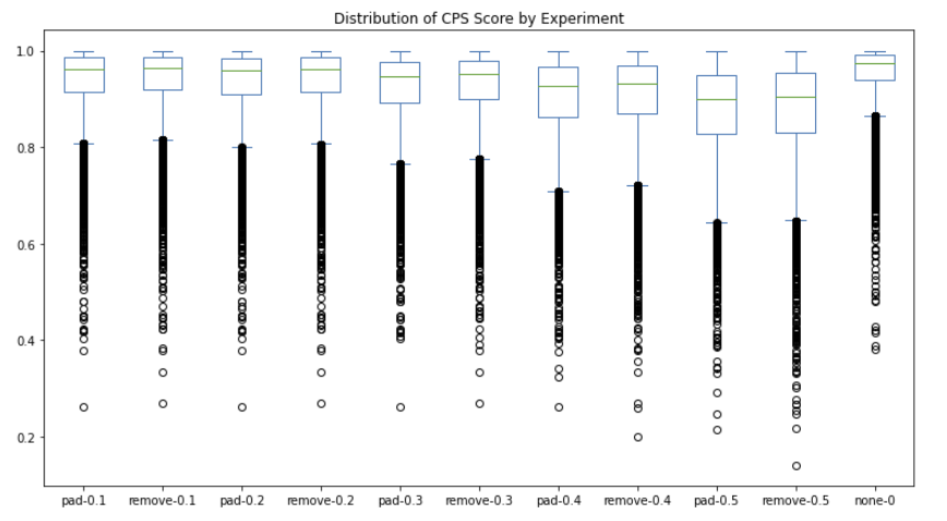Figure 5: Content preservation score distributions across various experimental settings for style threshold and masking strategy.

We found that for each incremental threshold value, token removal produces a slightly higher average CPS score than replacement with “[PAD]” token. We also see that regardless of the parameter combination, all cases result in a lower median similarity score than had no style-masking been applied at all (see far right column in Figure 5). This makes sense because the more tokens we mask, the more opportunity there is to erroneously remove a piece of content instead of a stylistic element.

The only true way to determine the “best” parameter combination is to look at how CPS correlates with human evaluated scores. However, since we don’t have access to manual evaluation scores, we select the combination that produces the highest outright CPS, which happens to be the case with no-style masking. For this reason, our CPS metric logic boils down to simply comparing SentenceBERT embeddings with cosine similarity, a similar landing place that others¹⁴⁵ have also arrived at.

Manual error analysis has revealed that our classifier-based attribution scores and style-token selection logic isn’t consistent, nor precise enough at isolating only stylistic elements. As a result, meaningful content tokens are mistakenly removed which hinders content preservation measurement more than just leaving all tokens in. We discuss these challenges further in the following sections.

Dependence on style classifier

Both of the metrics we’ve implemented depend on the availability of a well-fit style classification model. This requirement translates to the need for labeled data. And while this isn’t an issue for parallel TST tasks, it becomes a non-starter for the vast majority of style attributes where parallel data isn’t available.

Even when parallel data is available, it’s imperative that the trained model is performant. As we’ll see in a later section, data quality issues can lead to a classifier that learns patterns that are unrepresentative of the true target attribute and result in an error-prone model. Since the STI metric is built directly on classifier distribution outputs, it is apparent that errors with the model will surface as errors in the style metric.

Similarly, the CPS metric uses the word attributions that are derived from the classifier as the basis for style token masking. If the model learns incorrect relationships between features and style classes, errors in word attribution scores can cause the wrong tokens to be masked. Unfortunately, there is minimal tolerance for error in style masking because incorrectly masking a content-related token (e.g. proper noun) can completely alter the semantics, producing a very low similarity score.

Style token selection

While our method for isolating style tokens in a sentence is driven by robust, contextual feature importances, the actual token selection methodology has room for improvement.

To begin, feature importances are attributed per token. Because BERT uses a word-piece tokenizer, we can see fragments of the same word with drastically different attribution values. For example, in Figure 3 above, we find that the term “strikingly” is tokenized in to the word pieces “striking” and “##ly”, with the former attributed to ~15% importance and the latter just ~1%. Our current implementation considers these independently, and therefore applies a mask to just the root word alone. A considerable improvement would be to introduce logic that looks at combined scores for word pieces.

In addition, our method applies a “global” threshold to determine the amount of style (and therefore corresponding tokens) that are masked out. At a minimum, one token is always masked. This logic could be improved as there is likely a relationship between length of sentence and maximum token feature importance. There are also cases where a sentence doesn’t contain any style-related terms, and therefore masking one token incorrectly removes content by default.

Decoupling style from content

Our content preservation metric naively assumes that style can in fact be disentangled from content.

This remains an open question in the NLP research community⁶, but from our experience and research, it seems there is growing consensus that style is woven into the content of written language, and the degree to which it can be separated is highly attribute-dependent. For the attribute of subjectivity, we believe that style is (at least partially) separable from content. For example, removing subjective modifiers (e.g. adjectives and adverbs) can change the style of a sentence without unwanted impact to semantics.

However, the challenge arises when theory meets practice. As we’ve found, automated methods for disentangling stylistic elements are consistently fraught with error, especially when operating in the lexical space (i.e. masking tokens). Newer approaches to text style transfer propose the separation of style from semantics in latent space representations with both supervised and unsupervised methods. We are encouraged by these efforts and look forward to continued research on this topic.

Are these metrics better than BLEU?

While we believe the STI and CPS metrics enable a more nuanced evaluation of text style transfer output than a singular BLEU score, we cannot say if these metrics are “better” without some human evaluated baseline to compare against. A “better” evaluation metric is just one that correlates stronger with human judgment, as this is the ultimate goal of automated evaluation.

Unfortunately, conducting human evaluation is outside the scope of our current research endeavor, but we do propose this as future work to build upon. In particular, we suggest conducting human evaluation in accord with this paper as a means to produce reliable evaluation benchmarks.

It’s important to note that while human evaluation is the “best” means for evaluating generated text, it still isn’t without issue. That’s because determining if something is subjective vs. neutral is itself subjective. Subjective evaluation tasks likely lead to a higher degree of variability even among human reviewers.

Evaluating BART with STI & CPS

With our custom metrics defined, we utilize them to evaluate our fine-tuned BART model’s ability to neutralize subjective language on the held out test set. We calculate STI and CPS scores between both the source and generated text, as well as the source and ground truth target annotation. Comparing metrics across these pairs helps build intuition for their overall usefulness and enables us to isolate edge cases of unexpected performance.

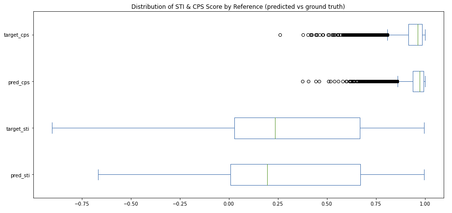Figure 6: Distribution of STI and CPS scores on the held out test set. “Pred” corresponds to scores between source and generated text, while “target” corresponds to scores between source and ground truth annotation.

Content Preservation Score (CPS)

CPS score is built on cosine similarity and so it naturally ranges from 0-1. Figure 6 highlights the strong, left-skewed distribution of both the source-to-target and source-to-prediction examples. This result makes sense because we expect input and output pairs to be largely similar in semantics as that is the essence of this task and dataset – to slightly modify style while retaining meaning.

We see very similar distributions between target and predicted samples, with the source-to-predicted pairs having slightly higher median CPS scores and a smaller standard deviation. As we’ll see, this finding hints at the conservative nature of our model (i.e. modest edits compared to human-made edits), as well as the perceptible data quality issues present in the full WNC corpus.

We analyze edge cases of mismatched performance between the model outputs and ground truths in Figure 7 below to better understand the strengths and weaknesses of our metrics.

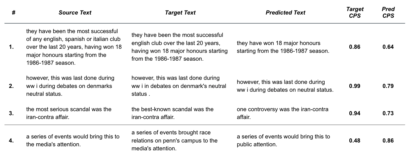
Figure 7: Sample WNC pairs that demonstrate common themes around the CPS metric. Specifically, cases where target_cps » predicted_cps (1-3) and target_cps « predicted_cps (4).

From Figure 7, we see that examples 1-3 highlight the scenario where the ground truth annotation preserves content much better (as defined by CPS) than the model’s output, and the opposite for example 4. These examples demonstrate common themes (numerically matched below) that we’ve found through our error analysis.

1. The BART model tends toward brevity - The trained seq2seq model has learned that omission of content is generally a good tactic for reducing subjectivity. This is seen in the example above where the model selects an abbreviated version of the input. Because the model omits part of the content (i.e. “being the most successful club”), our CPS metric punishes the score relative to the ground truth.
2. SentenceBERT penalizes missing content - As expected, SentenceBERT embedding similarity captures the omission of important words. In this example, the prediction is penalized for dropping the important subject “Denmark”.
3. CPS slips when style tokens are the difference - In contrast with example #2, our CPS metric struggles when the omitted words (“most serious”) are actually style related. In this example, CPS produces a disagreeably low score for the prediction as compared to the ground truth despite it largely retaining the semantic meaning. This demonstrates the imperative of isolating style elements from content. We tested removing these style-related terms (“most serious”) which resulted in a CPS score more representative of the semantic alignment.
4. Factual edits are out-of-scope - In this example, our model generated text produces a much higher CPS than the ground truth. This is due to the annotator’s introduction of new facts, or out-of-context information, that the model should not be expected to produce. We consider edits of this type to be outside the scope of our intended modeling task.

Overall, we see that our CPS metric has its strengths and weaknesses. We believe this metric is useful for providing a general indication of content preservation because low scores truly mark dissimilar content. However, this metric lacks marginal specificity and struggles to quantify small differences in content with accuracy.

Style Transfer Intensity (STI)

Unlike CPS, style transfer intensity ranges from -1 to 1 because movements away from the target style are penalized. We see from Figure 6 (above) and Figure 8 (below) that source-to-target and source-to-prediction STI distributions are very similar, which suggests the style transfer model is generally doing a good job of neutralizing text to resemble that of the ground truth.

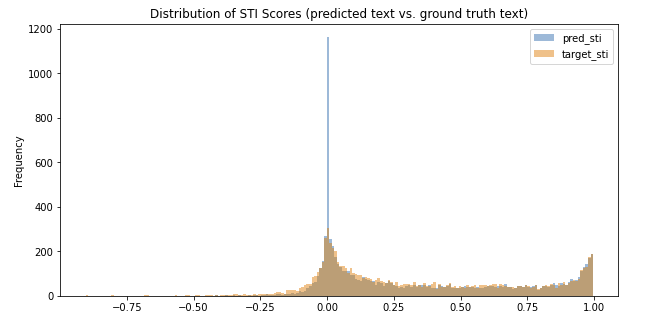Figure 8: Histogram of STI scores on held out test set. “Pred” corresponds to scores between source and generated text, while “target” corresponds to scores between source and ground truth annotation.

However, there is a clear discrepancy between the distributions at STI value of 0. Here we see a significant number of generations that result in no change in style – these are cases where we found the model simply repeats the input as output. This implies that model is conservative in nature (i.e. refrains from making unsure edits) and explains the lower median STI score for the source-to-target population (0.19 vs. 0.24)

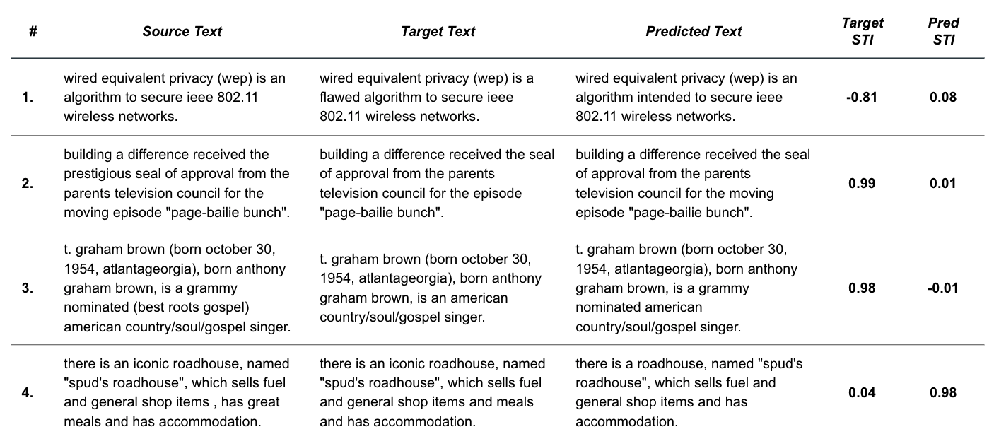Figure 9: Sample WNC pairs that demonstrate common themes around the STI metric. Specifcally, cases where target_sti < 0 (1), target_sti » pred_sti (2-3), and target_sti « pred_sti (4).

Like in the CPS analysis, we can look at edge cases shown in Figure 9 to highlight themes about model and metric quality.

1. Incorrect target annotations - Figure 8 reveals that there are examples where the ground truth STI score is negative – implying that the ground truth annotation is more subjective than the source, which we can verify by looking at this first example. We see that the target text introduces the subjective modifier “flawed”, which is clearly a labeling error. There are quite a few of these data quality issues that should be investigated and corrected in the dataset for future work.
2. BART can be partially correct - As shown here, there are many instances where the style transfer model correctly edits one instance of subjectivity in a sentence (e.g. removes “prestigious”), but misses additional occurrences (e.g. “moving”).
3. Classifier error surfaces in STI metric - As discussed previously, STI depends on the quality of the style classification model. This example shows where the classifier incorrectly associates “grammy nominated” as a subjective modifier, when in fact the modifier phrase consists of neutral content.
4. BART sometimes does better than ground truth - By inspecting cases where target_sti << pred_sti, we find examples where the fine-tuned style transfer model legitimately outperforms the ground truth – a hopeful insight into the potential usefulness of the model.

Interpreting the STI metric

Style transfer intensity, as defined above, produces a directional magnitude indicating the distributional shift between style classifications from an input and output text. While this is a useful metric, it is difficult to compare across examples because the value is not normalized. For example, an STI score of 0.1 appears to be a weak indication of style transfer. But if that score corresponds to a distribution shift from [0.1, 0.9] to [0.0, 1.0], it actually represents the maximum possible shift in style because the distribution only had little room for improvement. Therefore, what appears to be a low STI score actually captured 100% of the possible target style gap. It would make little sense to put this example on the same footing as a distribution shift from [0.9, 0.1] to [0.8, 0.2].

This highlights the fact that STI should be measured relative to the total potential for style transfer. For this reason, we recommend representing STI as a percentage of the total possible, directionally corrected STI gain. If the output text distribution moves closer towards the target style class, the metric represents the percentage of the possible target style distribution that was captured. If output text distribution moves further from the target style class, the metric represents the percentage of the possible source style distribution that was captured.

Wrapping up

In this post, we took a close look at what it means to comprehensively evaluate text style transfer and the associated challenges in doing so. We proposed a set of metrics that aim to quantify transferred style strength and content preservation. Through our metric development process, we got a first hand look at the tradeoffs that exist when substituting manual, human evaluation for an automated proxy.

Evaluating our BART model with the STI and CPS metrics revealed strengths and weaknesses of the metrics themselves, the dataset, and the model. We encourage further benchmarking of these metrics against human evaluated scores and recognize the need for cleaning up data quality concerns with the full WNC corpus (e.g. grammar, punctuation, & factual based-edits, labeling errors, incomplete ground truth annotations).

We’ve openly released our models (seq2seq, classification), datasets, and code to enable further experimentation with this text style transfer use case, and look forward to the continued progress on this exciting NLP task!

References